Territory of electrical information WEBSOR. Dynamic System State Variables

The system is called observable if in the formation of the output coordinates vector all components of the vector of state variables are involved. If none of the components of the vector affects the formation of the output of the system , then such a system will be unobservable.

Controllability and observability analysis is performed using controllability matrices and observability or using controllability gramians and observability.

Based on the matrices , , we form two auxiliary matrices

R = [ , , ..., n-1 ], D= [ , ,…, n -1 ]

Matrices R and D are called respectively controllability matrix and observability matrix systems. In the MATLAB package, they can be built using the commands ctrb and obsv.

For system (3.2) to be controllable, it is necessary that

it is sufficient that the controllability matrix has full rank rankR = n.

For system (3.2) to be observable, it is necessary and sufficient that the observability matrix has the full rank rankD=n.

In the case of systems with one input and one output of the matrix R and D square, so to check the controllability and observability, it is enough to calculate the determinants of the matrices R and D. If they are not equal to zero, then the matrices have full rank.

Lecture 4

Evaluation of static properties

Depending on the processes occurring in the ACS, two modes of operation of the ACS and its elements are distinguished: dynamic and static.

The transitional process corresponds to the dynamic mode of functioning of the ACS and their elements. This mode is given the most time in TAU. In dynamic mode, the values ​​that determine the state of the ACS and their elements change over time. Above, mathematical models of ACS in dynamic mode were presented in the form of differential equations n th (2.1) or in the form of equations of state (3.2, 3.3).

On the contrary, the steady-state process in the ACS corresponds to the static mode of operation, in which the quantities characterizing the state of the ACS do not change in time. To assess the ACS in a static (steady) mode, an indicator called control accuracy is used. This indicator is determined by the static characteristics of the ACS.

Rice. 4.1. Static characteristics of static and astatic systems

The static characteristic of the ACS represents the dependence of the steady value of the output parameter – y 0 from the input parameter – u 0 with a constant perturbation, or the dependence of the output parameter - y 0 in the steady state from perturbation– f with a constant input parameter. The ACS statics equations have the form or . In general, the equations can be non-linear. Consider the static characteristic of elements or ACS as a whole (Fig. 4.1) built according to the second equation. If the steady value of the error in the system depends on the steady value of the perturbation f, then the system is called static (Fig. 4.1, a), and if it does not depend, then astatic (Fig. 4.1, b).

The relative static error, or droop, of the system is

Also, droop can be characterized by a droop coefficient equal to the tangent of the slope of the static characteristic (Fig. 3.1, a).

The efficiency of the static control of the automatic control system in the steady state is evaluated by the so-called degree of control accuracy, which is equal to the ratio of the absolute static error of the non-automated control object (without the controller) to the absolute static error of the automatic system.

In some cases, a static error is undesirable, then they switch to astatic control or introduce compensatory effects on disturbances.

Study the theoretical material in educational literature:; and answer the following questions:

1. What variables in an electrical circuit are usually taken as state variables?

2. How many systems of equations make up when solving the problem by the method of state variables?

3. What dependencies are established in the first and second systems of equations when solving the problem by the method of state variables?

4. Which of the two systems is a system of differential equations, algebraic?

5. What methods are used to obtain state equations and output parameter equations?

When calculating the transient process using the state variable method, the following order is recommended:

1. Select state variables. In the circuits proposed for calculation, these are voltages on capacitive elements and currents in inductive coils.

2. Compose a system of differential equations for the first derivatives of state variables.

To do this, describe the post-switching circuit using Kirchhoff's laws and solve it with respect to the first derivatives of the state variables and depending on the variables , and emf sources. (in the proposed schemes, the emf source is the only one).

In matrix form, this system of differential equations of the 1st order will look like:

, (8.1)

where is the column of derivatives , ;

X– vector - column of state variables.

In chains of the second order:

is a square matrix of order n determined by the topology of the electrical circuit and the parameters of its elements. In chains of the second order, this matrix has the order 2´2.

The matrix is ​​a rectangular matrix of order , where n- chain order.

Matrix - column - is determined by emf sources. and sources of circuit currents and is called vector of input values.

3. Compose a system of algebraic equations for the desired variables, which are called weekend. These are currents in any branches of the circuit (except current) and voltages on any elements of the circuit (except voltage). The resulting algebraic equations establish relationships between output variables, on the one hand, and state variables and circuit voltage and current sources, on the other. In matrix form, this system of algebraic equations has the form

,

where is the vector of output values;

– matrices determined by the topology of the electrical circuit, the parameters of its elements and the number of required variables.

The state variable method (otherwise known as the state space method) is based on two equations written in matrix form.

The structure of the first equation is determined by the fact that it connects the matrix of the first time derivatives of the state variables with the matrices of the state variables themselves and external influences and, which are considered e. d.s. and source currents.

The second equation is algebraic in its structure and connects the matrix of output values ​​y with the matrices of state variables and external influences u.

Defining state variables, we note the following properties

1. As state variables in electrical circuits, one should choose currents in inductances and voltages on capacities, and not in all inductances and not on all capacities, but only for independent ones, i.e. those that determine the general order of the system of differential equations of the circuit.

2. The differential equations of the circuit with respect to the state variables are written in canonical form, i.e., they are represented as solved with respect to the first derivatives of the state variables with respect to time.

Note that only when currents k in independent inductances and voltages on independent capacitances are chosen as state variables, the first equation of the method of state variables will have the structure indicated above.

If we choose currents in branches with capacitances or currents in branches with resistances as state variables, as well as voltages on inductances or voltages on resistances, then the first equation of the method of state variables can also be represented in canonical form, i.e., solved with respect to the first time derivatives these quantities. However, the structure of their right-hand sides will not correspond to the definition given above, since they will also include the matrix of first derivatives of external influences

3. The number of state variables is equal to the order of the system of differential equations of the electrical circuit under study.

4. The choice of the states of currents and voltages as variables is also convenient because, according to the laws of switching (§ 13-1), it is these quantities that do not change abruptly at the moment of switching, i.e., they are the same for moments of time

5. State variables are called so because at each moment of time they set the energy state of the electrical circuit, since the latter is determined by the sum of expressions

6. Representation of equations in canonical form is very convenient when solving them on analog computers and for programming when solving them on digital computers. Therefore, such a representation is very important when solving these equations with the help of modern computer technology.

Let us show on the example of the circuit in Fig. 14-14 how equations are composed using the state variable method.

First, we obtain a system of differential equations corresponding to the first matrix equation of the method, and then we write it in matrix form. The algorithm for compiling these equations for any electrical circuit is as follows. First, equations are written according to Kirchhoff's laws or according to the method of loop currents; then state variables are selected and by differentiating the original equations and eliminating other variables, we obtain

the equations of the method of state variables are developed. This algorithm is very similar to that used in the classical method of calculating transients to obtain one resulting differential equation with respect to one of the variables

In special cases, when there are no capacitive circuits in the circuit, i.e. circuits, all branches of which contain capacitances, and there are no nodes with attached branches, each of which has inductances included, another algorithm can be specified. Without dwelling on it, we only note that it is based on the replacement of capacities by sources of e. d.s., inductances - current sources and the application of the superposition method.

For the circuit in Fig. 14-14 according to Kirchhoff's laws

(14-36)

Determining from the first equation, substituting into the third, replacing and representing the resulting differential equation in canonical form with respect to, we obtain:

Solving the second equation (14-36) with respect to , substituting according to the first equation (14-36) and substituting , we get:

Adding term by term (14-38) with multiplied by the equation (14-37) and determining from the result obtained, we get:

Let's rewrite equations (14-39) and (14-37) in matrix form:

(14-4°)

where for the circuit under consideration we have:

(14-42a)

In the general case, the first equation of the state variable method in matrix form can be written as

(14-43)

Matrices A and B in linear circuits depend only on the parameters of the circuit, i.e., they are constant values. At the same time, A is a square matrix of order and is called the main matrix of the circuit, matrix B is generally rectangular, of size is called the matrix of the connection between the input of the circuit and state variables, matrices are column matrices or vectors of state variables (size and external disturbances (size )

In the example under consideration, the matrix B turned out to be square of the second order, since the number of state variables is equal to the number of external perturbations

Let's move on to compiling the second equation of the method. Any of the quantities can be chosen as the output. Take, for example, as output three quantities

Their values ​​will be written through state variables and external perturbations directly from equations (14 36)

(14-44)

or in matrix form

or abbreviated

(14-46)

where for the circuit under consideration

and in the general case, the second equation of the method of state variables

The matrices C and D depend only on the circuit parameters. In the general case, these are rectangular matrices, respectively, of sizes , and C is called the matrix of connection of state variables with the output of the circuit, the matrix of direct connection of the input and output of the circuit (or system).

For a number of physical systems, D is a zero matrix, and the second term in (14-48) vanishes, since there are no immediate direct connection between the input and output of the system.

If we take, for example, current i and voltage as state variables and represent the differential equations for them in canonical form, then (omitting all intermediate transformations) the first of the equations of the method in matrix form will look like:

Thus, indeed, the first equation of the method of state variables will have the form (14-43) in matrix form only when choosing current and voltage as state variables

Turning to the solution of the matrix differential equation (14-43), first of all, we note that it is especially simplified if the square basic matrix A of the order is diagonal. Then all linear differential equations (14-43) are decoupled, i.e. the derivatives of the state variables each depend only on their state variable.

Let us first consider the solution of the linear inhomogeneous matrix differential equation (14-43) by the operator method. To do this, we transform it according to Laplace:

and the matrix-column of the initial values ​​of the state variables, i.e.

(14-53)

which do not change abruptly at the moment of switching, are given and equal to their values ​​at the moment

Let's rewrite (14-51):

where is the identity matrix of order .

To obtain a matrix of images of state variables, we multiply both parts (14-54) on the left by the inverse matrix

Passing back to the originals using the inverse Laplace transform, we get:

It is known from the operator method that

By analogy, writing the inverse Laplace transform in matrix form, we will have:

where is the transition matrix of the state of the system, otherwise called fundamental.

Thus, we find the original of the first term on the right side (14-56)

The inverse matrix is ​​determined by dividing the adjoint or reciprocal matrix by the determinant of the main matrix:

where is the equation

(14-61)

is the characteristic equation of the circuit under study.

The original of the second term on the right side (14-56) is found using the convolution theorem in matrix form

if put

Then based on (14-62)-(14-64)

and the general solution of the differential inhomogeneous matrix equation (14-43) based on (14-56), (14-59) and (14-65) will look like:

(14-66)

The first term of the right side (14-66) represents the values ​​of the state variables or the response of the circuit at zero input, i.e. In other words, it represents the first component of the free processes in the circuit due to non-zero initial values ​​of the state variables of the circuit, and therefore is a solution to the equation. The second term is the component of the chain reaction at, i.e., at the zero state of the chain.

The zero state of the chain is its state when the initial values ​​of all state variables are equal to zero. In other words, the second term (14-66) is the sum of the forced reaction of the chain arising under the influence of external influences and the second component of free processes

Equality (14-66) means that the reaction of the chain is equal to the sum of the reactions at zero input and zero state.

Based on (14-48) and (14-66) for the output values, we have.

If the state of the circuit is given not at the moment , but at the moment , then equalities (14-66) and (14-67) are generalized:

(14-68)

Example 14-5. For a branched chain of the second order, the equations of state are composed

under nonzero initial conditions and with the only source of e. d.s.

Find state variables.

Solution. Let us rewrite the equations of state in matrix form

Let us first find the first free components of the state variables at zero input. To do this, we will compose the matrix

To find the associated or reciprocal matrix, we replace each element in the previous matrix with its algebraic complement. We obtain the matrix

We transpose it by finding the adjoint or reciprocal matrix:

Let's find the matrix determinant

Based on (14-60), the inverse matrix will be:

Let us subject it to the inverse Laplace transform, taking into account the fact that for this it is necessary to subject each of its elements to the inverse Laplace transform. Based on (14-73), we obtain the transition matrix of the circuit state

For example,

For the transition matrix of the system state, we obtain:

For the first free components of the state variables, we have

Summing up the results obtained, we find the desired values ​​of the state variables:

Since the solution of equation (14-43) was obtained above and given by the formula (14-66), then to check the correctness of the solution (14-66) and use it to calculate the matrix of state variables, you can first by directly substituting (14-66) into ( 14-43) make sure that the latter turns into an identity. To do this, you only need to first calculate by differentiating (14-66). In doing so, we get:

Now it is easy to verify directly that (14-66) is indeed a solution of the matrix differential equation

Note that the transition matrix of the state of the system allows us to find in the state space, i.e., in the space, the number of dimensions of which is equal to the number of components of the vector of state variables, the movement starting from some initial position (at or at ) and the vector contains significant information, since simultaneously describes all state variables, i.e. functions of time.

Multiple regression is not the result of a transformation of the equation:

-
;

-
.

Linearization implies a procedure...

- bringing the equation of multiple regression to the steam room;

+ bringing a nonlinear equation to a linear form;

- reduction of a linear equation to a non-linear form;

- reduction of a nonlinear equation with respect to parameters to an equation that is linear with respect to the result.

Remains do not change;

The number of observations decreases

In a standardized multiple regression equation, the variables are:

Initial variables;

Standardized parameters;

Mean values ​​of initial variables;

standardized variables.

One method for assigning numeric values ​​to dummy variables is. . .

+– ranking;

Alignment of numerical values ​​in ascending order;

Alignment of numerical values ​​in descending order;

Finding the mean.

The matrix of paired correlation coefficients displays the values ​​of the pairwise linear correlation coefficients between. . . .

Variables;

parameters;

Parameters and variables;

Variable and random factors.

The method for estimating the parameters of models with heteroscedastic residuals is called the ____________ least squares method:

Ordinary;

Indirect;

generalized;

Minimum.

The regression equation is given. Define the model specification.

Polynomial Pair Regression Equation;

Linear simple regression equation;

Polynomial equation of multiple regression;

Linear multiple regression equation.

In a standardized equation, the free term is ….

Equals 1;

Equal to the coefficient of multiple determination;

Equal to the multiple correlation coefficient;

Missing.

Factors are included as dummy variables in the multiple regression model.

Having probabilistic values;

Having quantitative values;

Not having qualitative values;

Not having quantitative values.

The factors of the econometric model are collinear if the coefficient ...

Correlations between them modulo more than 0.7;

The determinations between them are greater than 0.7 in absolute value;

The determinations between them are less than 0.7 in absolute value;

The generalized least squares method differs from the usual least squares method in that, when using GLS ...

The original levels of the variables are converted;

Remains do not change;

The remainder is equal to zero;

The number of observations decreases.

The sample size is determined ...

The numerical value of the variables selected in the sample;

The volume of the general population;

The number of parameters for independent variables;

The number of result variables.

11. Multiple regression is not the result of a transformation of the equation:

+-
;

-
;

-
.

The initial values ​​of the dummy variables assume the values ​​...

quality;

Quantitatively measurable;

The same;

Values.

The generalized least squares method implies ...

Variable conversion;

Transition from multiple regression to pair regression;

Linearization of the regression equation;

Two-stage application of the least squares method.

The linear equation of multiple regression has the form . Determine which factor or :

+- , since 3.7>2.5;

They have the same effect;

- , since 2.5>-3.7;

According to this equation, it is impossible to answer the question posed, since the regression coefficients are incomparable among themselves.

The inclusion of a factor in the model is advisable if the regression coefficient for this factor is ...

Zero;

insignificant;

essential;

Insignificant.

What is transformed when applying the generalized least squares method?

Standardized regression coefficients;

Dispersion of the effective feature;

Initial levels of variables;

Dispersion of a factor sign.

A study is being made of the dependence of the production of an enterprise employee on a number of factors. An example of a dummy variable in this model would be ______ employee.

Age;

The level of education;

Wage.

The transition from point estimation to interval estimation is possible if the estimates are:

Effective and insolvent;

Inefficient and wealthy;

Efficient and unbiased;

Wealthy and displaced.

A matrix of pairwise correlation coefficients is built to identify collinear and multicollinear …

parameters;

Random factors;

significant factors;

results.

Based on the transformation of variables using the generalized least squares method, we obtain a new regression equation, which is:

Weighted regression in which variables are taken with weights
;

;

Nonlinear regression in which variables are taken with weights
;

Weighted regression in which variables are taken with weights .

If the calculated value of the Fisher criterion is less than the tabular value, then the hypothesis of the statistical insignificance of the equation ...

Rejected;

insignificant;

accepted;

Not essential.

If the factors are included in the model as a product, then the model is called:

total;

derivative;

Additive;

Multiplicative.

The regression equation that relates the resulting feature to one of the factors with the value of other variables fixed at the average level is called:

Multiple;

essential;

Private;

Insignificant.

Regarding the number of factors included in the regression equation, there are ...

Linear and non-linear regression;

Direct and indirect regression;

Simple and multiple regression;

Multiple and multivariate regression.

The requirement for regression equations, the parameters of which can be found using the least squares method, is:

Equality to zero of the values ​​of the factor attribute4

Non-linearity of parameters;

Equality to zero of the average values ​​of the resulting variable;

Linearity of parameters.

The least squares method is not applicable for ...

Linear equations of pair regression;

Polynomial multiple regression equations;

Equations that are non-linear in terms of the estimated parameters;

Linear equations of multiple regression.

When dummy variables are included in the model, they are assigned ...

Null values;

Numeric labels;

Same values;

Quality labels.

If there is a non-linear relationship between economic indicators, then ...

It is not practical to use the specification of a non-linear regression equation;

It is advisable to use the specification of a non-linear regression equation;

It is advisable to use the specification of a linear paired regression equation;

It is necessary to include other factors in the model and use a linear multiple regression equation.

The result of the linearization of polynomial equations is ...

Nonlinear Pair Regression Equations;

Linear equations of pair regression;

Nonlinear multiple regression equations;

Linear equations of multiple regression.

In the standardized multiple regression equation
0,3;
-2.1. Determine which factor or has a stronger effect on :

+- , since 2.1>0.3;

According to this equation, it is impossible to answer the question posed, since the values ​​of the “pure” regression coefficients are unknown;

- , since 0.3>-2.1;

According to this equation, it is impossible to answer the question posed, since the standardized coefficients are not comparable with each other.

The factor variables of a multiple regression equation converted from qualitative to quantitative are called ...

anomalous;

Multiple;

Paired;

Fictitious.

Estimates of the parameters of the linear equation of multiple regression can be found using the method:

Medium squares;

The largest squares;

Normal squares;

Least squares.

The main requirement for the factors included in the multiple regression model is:

Lack of relationship between result and factor;

Lack of relationship between factors;

Lack of linear relationship between factors;

The presence of a close relationship between factors.

Dummy variables are included in the multiple regression equation to take into account the effect of features on the result ...

quality character;

quantitative nature;

of a non-essential nature;

Random character.

From a pair of collinear factors, the econometric model includes the factor

Which, with a fairly close connection with the result, has the greatest connection with other factors;

Which, in the absence of connection with the result, has the maximum connection with other factors;

Which, in the absence of a connection with the result, has the least connection with other factors;

Which, with a fairly close relationship with the result, has a smaller relationship with other factors.

Heteroskedasticity refers to...

The constancy of the variance of the residuals, regardless of the value of the factor;

The dependence of the mathematical expectation of the residuals on the value of the factor;

Dependence of the variance of residuals on the value of the factor;

Independence of the mathematical expectation of the residuals from the value of the factor.

The value of the residual variance when a significant factor is included in the model:

Will not change;

will increase;

will be zero;

Will decrease.

If the specification of the model displays a non-linear form of dependence between economic indicators, then the non-linear equation ...

regressions;

determinations;

Correlations;

Approximations.

The dependence is investigated, which is characterized by a linear multiple regression equation. For the equation, the value of the tightness of the relationship between the resulting variable and a set of factors is calculated. As this indicator, a multiple coefficient was used ...

Correlations;

elasticity;

regressions;

Determinations.

A model of dependence of demand on a number of factors is being built. The dummy variable in this multiple regression equation is not _________consumer.

Family status;

The level of education;

For an essential parameter, the calculated value of the Student's criterion ...

More than the table value of the criterion;

Equal to zero;

Not more than the tabular value of the Student's criterion;

Less than the table value of the criterion.

An LSM system built to estimate the parameters of a linear multiple regression equation can be solved...

Moving average method;

The method of determinants;

Method of first differences;

Simplex method.

An indicator characterizing how many sigmas the result will change on average when the corresponding factor changes by one sigma, with the level of other factors unchanged, is called ____________ regression coefficient

standardized;

Normalized;

Aligned;

Centered.

The multicollinearity of the factors of the econometric model implies…

The presence of a non-linear relationship between the two factors;

The presence of a linear relationship between more than two factors;

Lack of dependence between factors;

The presence of a linear relationship between the two factors.

Generalized least squares is not used for models with _______ residuals.

Autocorrelated and heteroscedastic;

homoscedastic;

heteroskedastic;

Autocorrelated.

The method for assigning numeric values ​​to dummy variables is not:

Ranging;

Assignment of digital labels;

Finding the average value;

Assignment of quantitative values.

Normally distributed residues;

Homoscedastic residues;

Autocorrelation residuals;

Autocorrelations of the resulting trait.

The selection of factors in a multiple regression model using the inclusion method is based on a comparison of values ​​...

The total variance before and after including the factor in the model;

Residual variance before and after including random factors in the model;

Variances before and after inclusion of the result in the model;

Residual variance before and after inclusion of factor model.

The generalized least squares method is used to correct...

Parameters of the nonlinear regression equation;

The accuracy of determining the coefficient of multiple correlation;

Autocorrelations between independent variables;

Heteroskedasticity of residuals in the regression equation.

After applying the generalized least squares method, it is possible to avoid _________ residuals

heteroskedasticity;

Normal distribution;

Equal to zero sums;

Random character.

Dummy variables are included in the ____________regression equations

Random;

steam room;

Indirect;

Multiple.

The interaction of the factors of the econometric model means that…

The influence of factors on the resulting feature depends on the values ​​of another non-collinear factor;

The influence of factors on the resulting attribute increases, starting from a certain level of factor values;

Factors duplicate each other's influence on the result;

The influence of one of the factors on the resulting attribute does not depend on the values ​​of the other factor.

Topic Multiple Regression (Problems)

The regression equation, built on 15 observations, has the form:

Missing values ​​as well as confidence interval for

with a probability of 0.99 are:

The regression equation, built on 20 observations, has the form:

with a probability of 0.9 are:

The regression equation, built on 16 observations, has the form:

Missing values ​​as well as confidence interval for with a probability of 0.99 are:

The regression equation in a standardized form is:

The partial elasticity coefficients are equal to:

The standardized regression equation is:

The partial elasticity coefficients are equal to:

The standardized regression equation is:

The partial elasticity coefficients are equal to:

The standardized regression equation is:

The partial elasticity coefficients are equal to:

The standardized regression equation is:

The partial elasticity coefficients are equal to:

Based on 18 observations, the following data were obtained:

;
;
;
;

are equal:

Based on 17 observations, the following data were obtained:

;
;
;
;

Values ​​of the adjusted coefficient of determination, partial coefficients of elasticity and parameter are equal:

Based on 22 observations, the following data were obtained:

;
;
;
;

Values ​​of the adjusted coefficient of determination, partial coefficients of elasticity and parameter are equal:

Based on 25 observations, the following data were obtained:

;
;
;
;

Values ​​of the adjusted coefficient of determination, partial coefficients of elasticity and parameter are equal:

Based on 24 observations, the following data were obtained:

;
;
;
;

Values ​​of the adjusted coefficient of determination, partial coefficients of elasticity and parameter are equal:

Based on 28 observations, the following data were obtained:

;
;
;
;

Values ​​of the adjusted coefficient of determination, partial coefficients of elasticity and parameter are equal:

Based on 26 observations, the following data were obtained:

;
;
;
;

Values ​​of the adjusted coefficient of determination, partial coefficients of elasticity and parameter are equal:

In the regression equation:

Restore missing characteristics; construct a confidence interval for with a probability of 0.95 if n=12

Knowing the response of the circuit to a single perturbing action, i.e. the transient conductivity function or (and) the voltage transient function , you can find the response of the circuit to the action of an arbitrary shape. The basis of the method - the method of calculation using the Duhamel integral - is the principle of superposition.

When using the Duhamel integral to separate the variable over which integration is performed and the variable that determines the time at which the current in the circuit is determined, the first is usually denoted as , and the second - as t.

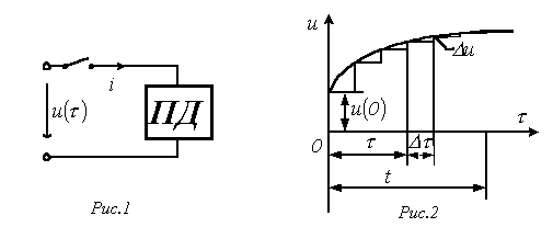
Let at the moment of time to the circuit with zero initial conditions (passive two-terminal network PD in fig. 1) a source with an arbitrary voltage is connected. To find the current in the circuit, we replace the original curve with a step curve (see Fig. 2), after which, taking into account that the circuit is linear, we sum the currents from the initial voltage jump and all voltage steps up to the moment t, which come into action with a time delay.

At time t, the component of the total current, determined by the initial voltage jump , is equal to .

There is a voltage jump at the moment , which, taking into account the time interval from the beginning of the jump to the point in time t of interest, will determine the current component .

The total current at time t is obviously equal to the sum of all current components from individual voltage surges, taking into account, i.e.

Replacing the finite time increment interval with an infinitely small one, i.e. passing from the sum to the integral, we write

.

(1)

Relation (1) is called the Duhamel integral.

It should be noted that the voltage can also be determined using the Duhamel integral. In this case, in (1) instead of the transient conductivity, the transient function with respect to voltage will enter.

Calculation sequence using
Duhamel integral

As an example of using the Duhamel integral, let us determine the current in the circuit in Fig. 3 calculated in the previous lecture using the inclusion formula.

Initial data for calculation: , , .

The result obtained is similar to the current expression defined in the previous lecture based on the inclusion formula.

State variables method

The electromagnetic state equations are a system of equations that determine the operating mode (state) of an electrical circuit.

The method of state variables is based on the ordered compilation and solution of a system of first-order differential equations that are resolved with respect to derivatives, i.e. are written in the form most convenient for the application of numerical integration methods implemented by means of computer technology.

The number of state variables, and consequently, the number of state equations is equal to the number of independent energy storage devices.

There are two main requirements for the equations of state:

Independence of equations;

The ability to restore based on state variables (variables with respect to which state equations are written) of any other variables.

The first requirement is satisfied by a special technique for compiling the equations of state, which will be discussed below.

To fulfill the second requirement, it is necessary to take flux links (currents in branches with inductive elements) and charges (voltages) on capacitors as state variables. Indeed, knowing the law of change of these variables in time, they can always be replaced by sources of EMF and current with known parameters. The rest of the circuit turns out to be resistive, and therefore, it is always calculated with known parameters of the sources. In addition, the initial values ​​of these variables are independent, i.e. in the general case are calculated easier than others.

When calculating by the method of state variables, in addition to the state equations themselves, linking the first derivatives and with the variables themselves and sources of external influences - EMF and current, it is necessary to compose a system of algebraic equations that connect the desired values ​​with state variables and sources of external influences.

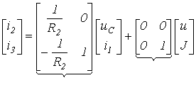
Thus, the complete system of equations in matrix form has the form

;

(2)

.

(3)

Here and are the columnar matrices, respectively, of the state variables and their first time derivatives; - matrix-column of sources of external influences; - columnar matrix of output (desired) values; - square dimension n x n(where n is the number of state variables) a parameter matrix, called the Jacobi matrix; - rectangular matrix of connection between sources and state variables (the number of rows is n, and columns - the number of sources m); - a rectangular matrix of connection of state variables with the desired values ​​(the number of rows is equal to the number of sought values ​​k, and the columns are n); - rectangular dimension to x m input-output connection matrix.

The initial conditions for equation (2) are given by the vector of initial values ​​(0).

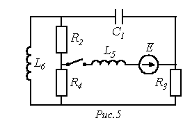
As an example of compiling equations of state, consider the circuit in Fig. 4a, in which it is required to determine the currents and .

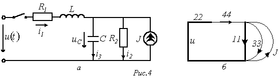
According to Kirchhoff's laws, for this circuit we write

;

(5)

A matrix equation of the form (3) follows from relations (4) and (6):

The vector of initial values ​​(0)= .

The direct use of Kirchhoff's laws when compiling equations of state for complex circuits can be difficult. In this regard, a special technique for orderly compiling the equations of state is used.

Technique for compiling equations of state

This technique includes the following main steps:

1. A directed graph of the circuit is compiled (see Fig. 4, b), on which a tree is allocated, covering all capacitors and voltage sources (EMF). Resistors are included in the tree as needed: to cover all nodes in the tree. The communication branch includes inductors, current sources and the remaining resistors.

2. The numbering of the branches of the graph (and the elements in the circuit) is carried out in the following sequence: the sections of the graph (circuit) with capacitors are numbered first, then the resistors included in the tree, the next are the communication branches with resistors and, finally, the branches with inductive elements ( see Fig. 4b).

3. A table is compiled describing the connection of elements in the chain. The first line of the table (see Table 1) lists the capacitive and resistive elements of the tree, as well as voltage sources (EMF). The first column lists the resistive and inductive elements of the communication branches, as well as the current sources.

Table 1 . Connection table

The procedure for filling the table consists in successively mentally closing the branches of the tree with the help of connection branches until a contour is obtained, followed by bypassing the latter according to the orientation of the corresponding connection branch. With the "+" sign, branches of the graph are written, the orientation of which coincides with the direction of bypassing the contour, and with the "-" sign, branches that have the opposite orientation are written.

The table is sorted by columns and rows. In the first case, equations are obtained according to the first Kirchhoff law, in the second - according to the second.

In the case under consideration (the equality is trivial)

,

whence, in accordance with the numbering of currents in the original circuit

.

When painting the connection table in rows, the voltages on the passive elements must be taken with signs opposite to those in the table:

(7)

These equations coincide with relations (6) and (5), respectively.

From (7) it immediately follows

.

Thus, equations similar to those compiled above using Kirchhoff's laws are obtained in a formalized way.

Literature

1. Bessonov L.A. Theoretical foundations of electrical engineering: Electrical circuits. Proc. for students of electrical, energy and instrument-making specialties of universities. –7th ed., revised. and additional –M.: Higher. school, 1978. -528s.
2. Matkhanov P.N. Fundamentals of electrical circuit analysis. Linear chains.: Proc. for electrical engineering radio engineering specialist. universities. 3rd ed., revised. and additional –M.: Higher. school, 1990. -400s.

Control questions and tasks

BUT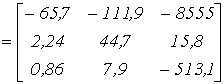
AT