Say you want to compare versions of a workbook, analyze a workbook for problems or inconsistencies, or see links between workbooks or worksheets. If Microsoft Office 365 or Office Professional Plus 2013 is installed on your computer, the Spreadsheet Inquire add-in is available in Excel.
You can use the commands in the Inquire tab to do all these tasks, and more. The Inquire tab on the Excel ribbon has buttons for the commands described below.
If you don't see the Inquire tab in the Excel ribbon, see Turn on the Spreadsheet Inquire add-in .
Compare two workbooks
The Compare Files command lets you see the differences, cell by cell, between two workbooks. You need to have two workbooks open in Excel to run this command.
Results are color coded by the kind of content, such as entered values, formulas, named ranges, and formats. There"s even a window that can show VBA code changes line by line. Differences between cells are shown in an easy to read grid layout, like this:

The Compare Files command uses Microsoft Spreadsheet Compare to compare the two files. In Windows 8, you can start Spreadsheet Compare outside of Excel by clicking Spreadsheet Compare on the Apps screen. In Windows 7, click the Windows Start button and then > All programs > Microsoft Office 2013 > Office 2013 Tools > Spreadsheet Compare 2013.
To learn more about Spreadsheet Compare and comparing files, read Compare two versions of a workbook .
Analyze a workbook
The Workbook Analysis command creates an interactive report showing detailed information about the workbook and its structure, formulas, cells, ranges, and warnings. The picture here shows a very simple workbook containing two formulas and data connections to an Access database and a text file.

Show workbook links
Workbooks connected to other workbooks through cell references can get confusing. Use the to create an interactive, graphical map of workbook dependencies created by connections (links) between files. The types of links in the diagram can include other workbooks, Access databases, text files, HTML pages, SQL Server databases, and other data sources. In the relationship diagram, you can select elements and find more information about them, and drag connection lines to change the shape of the diagram.
This diagram shows the current workbook on the left and the connections between it and other workbooks and data sources. It also shows additional levels of workbook connections, giving you a picture of the data origins for the workbook.

Show worksheet links
Got lots of worksheets that depend on each other? Use the to create an interactive, graphical map of connections (links) between worksheets both in the same workbook and in other workbooks. This helps give you a clearer picture of how your data might depend on cells in other places.
This diagram shows the relationships between worksheets in four different workbooks, with dependencies between worksheets in the same workbook as well as links between worksheets in different workbooks. When you position your pointer over a node in the diagram, such as the worksheet named "West" in the diagram, a balloon containing information appears.

Show cell relationships
To get a detailed, interactive diagram of all links from a selected cell to cells in other worksheets or even other workbooks, use the Cell Relationship tool. These relationships with other cells can exist in formulas, or references to named ranges. The diagram can cross worksheets and workbooks.
This diagram shows two levels of cell relationships for cell A10 on Sheet5 in Book1.xlsx. This cell is dependent on cell C6 on Sheet 1 in another workbook, Book2.xlsx. This cell is a precedent for several cells on other worksheets in the same file.

To learn more about viewing cell relationships, read See links between cells .
Clean excess cell formatting
Ever open a workbook and find it loads slowly, or has become huge? It might have formatting applied to rows or columns you aren't aware of. Use the Clean Excess Cell Formatting command to remove excess formatting and greatly reduce file size. This helps you avoid "spreadsheet bloat," which improves Excel's speed.
Manage passwords
If you"re using the Inquire features to analyze or compare workbooks that are password protected, you"ll need to add the workbook password to your password list so that Inquire can open the saved copy of your workbook. Use the Workbook Passwords command on the Inquire tab to add passwords, which will be saved on your computer. These passwords are encrypted and only accessible by you.
Need to compare two Microsoft Excel files? Here are two easy ways to do it.
There are many reasons why you might want to take one Excel document and compare it to another. This can be a labor intensive task.
it requires a lot of concentration, but there are ways to make your life easier.
Do you need to take a close look by hand or do you want Excel to do some heavy lifting
on your behalf, here are two easy ways to compare multiple sheets.
How to Compare Excel Files
Excel allows users to display two versions of a document at once to quickly distinguish between them:
- First, open the workbooks to be compared.
- Switch to View > Window > Side View.
Comparing Excel files by eye
To get started, open Excel and any workbooks you want to compare. We can use the same technique to compare sheets in the same document
or completely different files.
If more than one sheet is received from the same book, it must be separated in advance. To do this, go to View > Window > New Window.

This won't split the individual sheets permanently, just open a new instance of your document.

This menu will list all tables that are currently open. If you only have two open, they will be selected automatically.

Make your choice and click Good. You will see both tables appear on the screen.

If it's more convenient you can use Arrange everything button to switch between vertical and horizontal configuration.

One important option to be aware of is Synchronous scrolling switching.

Enabling this setting ensures that when one window scrolls, the other will move in sync. This is important if you are working with a large table.
and you want to keep testing one against the other. If for some reason the two sheets are not aligned, just click Reset window position.
Comparing Excel Files Using Conditional Formatting
In many cases, the best way to compare two spreadsheets may be to simply display them at the same time. However, it is possible to automate the process somewhat.
Using Conditional Formatting
We can check Excel for discrepancies between two sheets. This can save a lot of time if all you need to find are the differences between one version and another.
For this method, we need to make sure that the two sheets we are working with are part of the same workbook. To do this, right-click on the sheet name you want to transfer and select Move or copy.

Here you can use the drop down menu to decide which document it will be pasted into.

Select all the cells that are filled in on the worksheet where you want any differences to be highlighted. A quick way to do this is to click on the cell in the top left corner and then use the shortcut
Ctrl+Shift+End.
Switch to Home> Styles> Conditional Formatting> New Rule.

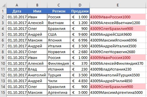
Choose Use a formula to determine which cells to format and enter the following:
A1sheet_name!A1
Just don't forget to lay out "sheet_name" for any other sheet name. This formula only checks when a cell on one sheet does not exactly match a corresponding cell on another sheet, and flags each instance.

Above you can see the results. All cells containing changes have been highlighted in red, making it quick and easy to compare two sheets.
Let Excel do the hard work
The above technique demonstrates one way you can let Excel handle some of the heavy lifting. Even if you pay close attention, chances are you might miss a change if you do this task manually. Thanks to conditional formatting, you can be sure that nothing is leaking onto the network.
Excel is good at monotonous and detail oriented work. Once you get the hang of it, you can save yourself some time and effort by using techniques like conditional formatting and a little ingenuity.
Do you have any advice for comparing documents in Excel? Or do you need help with the processes in this guide? In any case, why not join the conversation in the comments section below?
Question from user
Hello!
I have one problem, and for the third day I have been racking my brains - I don’t know how to complete it. There are 2 tables (about 500-600 rows in each), you need to take a column with the name of the product from one table and compare it with the name of the product from the other, and if the products match, copy and substitute the value from table 2 to table 1. Intricately explained , but I think you will understand the task from the photo ( approx. : the photo was cut out by censors, after all, personal information).
Thank you in advance. Andrey, Moscow.
Good day everyone!
What you have described is a fairly popular task that is relatively easy and quick to solve using Excel. It is enough to drive your two tables into the program, and use the VLOOKUP function. More on her work below...
An example of working with the VLOOKUP function
As an example, I took two small plates, they are presented in the screenshot below. In the first table (columns A, B- product and price) no data for the column B; in the second - both columns are filled (product and price). Now you need to check the first columns in both tables and automatically, if a match is found, copy the price to the first plate. Seems like a simple problem...

How to do it...
Place the mouse pointer in a cell B2- that is, in the first cell of the column, where we have no value and write the formula:
=VLOOKUP(A2 ;$E$1:$F$7 ;2 ;FALSE )
A2- value from the first column of the first table (what we will look for in the first column of the second table);
$E$1:$F$7- a fully selected second table (in which we want to find and copy something). Pay attention to the "$" sign - it is necessary so that when copying the formula, the cells of the selected second table do not change;
2 - the number of the column from which we will copy the value (note that our selected second table has only 2 columns. If it had 3 columns, then the value could be copied from the 2nd or 3rd column);
FALSE- we are looking for an exact match (otherwise the first similar one will be substituted, which obviously does not suit us).

Actually, you can adjust the finished formula to your needs by slightly changing it. The result of the formula is shown in the picture below: the price was found in the second table and substituted in auto mode. Everything is working!

To set the price for other items of goods - just stretch (copy) the formula to other cells. An example is below.

After that, as you can see, the first columns of the tables will be compared: from the rows where the cell values matched, the necessary data will be copied and substituted. In general, it is clear that tables can be much larger!

Note: I must say that the VLOOKUP function is quite demanding on computer resources. In some cases, with an excessively large document, it may take quite a long time to compare the tables. In these cases, it is worth considering either other formulas or completely different solutions (each case is individual).
That's all, good luck!
After installing the add-on, you will have a new tab with a function call command. When you click on a command Range Comparison a dialog box appears for entering parameters.
This macro allows you to compare tables of any size and with any number of columns. Tables can be compared on one, two or three columns at a time.
The dialog box is divided into two parts: left for the first table and right for the second.
To compare tables, do the following:
- Specify table ranges.
- Set a checkbox (daw/checkmark) under the selected range of tables if the table includes a header (header row).
- Select the columns of the left and right tables to be compared (if the table ranges do not include headers, the columns will be numbered).
- Specify the type of comparison.
- Select the output option.
Table comparison type
 The program allows you to select several types of table comparison:
Find rows in one table that are missing in another table
When this type of comparison is selected, the program looks for rows in one table that are missing in another. If you compare tables by several columns, then the result of the work will be rows in which there is a difference in at least one of the columns.
Find matching lines
When this type of comparison is selected, the program finds rows that match in the first and second tables. Matching rows are those in which the values in the selected comparison columns (1, 2, 3) of one table completely match the values of the columns of the second table.
An example of the program in this mode is shown on the right in the picture.
Match tables based on selected
In this comparison mode, in front of each row of the first table (selected as the main one), the data of the matching row of the second table is copied. If there are no matching rows, the row opposite the main table remains empty.
Comparing tables with four or more columns
If you lack the functionality of the program and need to match tables on four or more columns, then you can get around this as follows:
- Create an empty column in the tables.
- In new columns using the formula = CONNECT concatenate the columns you want to compare against.
So you will end up with 1 column containing the values of multiple columns. Well, you already know how to match one column.
Perhaps everyone who works with data in Excel is faced with the question of how to compare two columns in Excel for matches and differences. There are several ways to do this. Let's take a closer look at each of them.
How to compare two columns in Excel row by row
When comparing two columns of data, it is often necessary to compare the data in each individual row for matches or differences. We can make such an analysis using the function . Let's see how it works in the examples below.
Example 1: How to compare two columns for matches and differences in the same row
In order to compare the data in each row of two columns in Excel, we write a simple formula. The formula should be inserted into each row in the adjacent column, next to the table in which the main data is located. Having created a formula for the first row of the table, we can stretch / copy it to the rest of the rows.
In order to check if two columns of one row contain the same data, we need a formula:
=IF(A2=B2, “Match”, “”)
The formula that determines the differences between the data of two columns in one row will look like this:
=IF(A2<>B2; "Do not match"; “”)
We can fit the check for matches and differences between two columns on one line in one formula:
=IF(A2=B2, “match”, “do not match”)
=IF(A2<>B2; "Do not match"; "Match")
An example calculation result might look like this:
To compare data in two columns of the same row, case sensitive, use the formula:
=IF(EXACT(A2,B2), “Match”, “Unique”)
How to compare multiple columns for matches in one row in Excel
Excel has the ability to compare data in multiple columns of the same row using the following criteria:
- Find rows with the same values in all columns of the table;
- Find rows with the same values in any two columns of the table;
Example1. How to find matches in one row in multiple columns of a table
Imagine that our table consists of several columns with data. Our task is to find rows in which the values match in all columns. The functions of Excel and . The formula for determining matches would be:
=IF(AND(A2=B2,A2=C2), “match”, ” “)
If our table has a lot of columns, then it will be easier to use the function in combination with:
=IF(COUNTIF($A2:$C2,$A2)=3;”match”;” “)
In the formula, “5” indicates the number of columns of the table for which we created the formula. If your table has more or less columns, then this value should be equal to the number of columns.
Example 2: How to find matches in one row in any two columns of a table
Imagine that our task is to identify from a table with data in several columns those rows in which the data matches or repeats in at least two columns. The functions and will help us with this. Let's write a formula for a table consisting of three columns with data:
=IF(OR(A2=B2;B2=C2;A2=C2);”match”;” “)
In cases where there are too many columns in our table, our formula with a function will be very large, since in its parameters we need to specify the match criteria between each column of the table. An easier way, in this case, is to use the .
=IF(COUNTIF(B2:D2,A2)+COUNTIF(C2:D2,B2)+(C2=D2)=0; “Unique string”; “Not unique string”)
=IF(COUNTIF($B:$B,$A5)=0, “No matches in column B”, “There are matches in column B”)
This formula checks the values in column B against the cell data in column A.
If your table has a fixed number of rows, you can specify a clear range in the formula (for example, $B2:$B10). This will speed up the formula.
How to compare two columns in Excel for matches and highlight with color
When we are looking for matches between two columns in Excel, we may need to visualize the found matches or differences in the data, for example by using color highlighting. The easiest way to highlight matches and differences is to use Conditional Formatting in Excel. Let's see how to do it in the examples below.
Finding and highlighting matches by color in multiple columns in Excel
In cases where we need to find matches in several columns, then for this we need:
- Select columns with data in which you want to calculate matches;
- On the “Home” tab on the Toolbar, click on the menu item “Conditional Formatting” -> “Cell Selection Rules” -> “Duplicate Values”;
- In the pop-up dialog box, select the item “Repeated” in the left drop-down list, in the right drop-down list, select which color the repeated values will be highlighted. Click the "OK" button:
- After that, matches will be highlighted in the selected column:

Find and highlight matching rows in Excel
Searching for matching cells with data in two or more columns and searching for matches of entire rows with data are different concepts. Take a look at the two tables below:
The tables above contain the same data. Their difference is that in the example on the left, we were looking for matching cells, and on the right, we found entire repeating rows with data.
Consider how to find matching rows in a table:
- To the right of the table with data, we will create an auxiliary column, in which, opposite each row with data, we will put down a formula that combines all the values of the table row into one cell:
=A2&B2&C2&D2
In the auxiliary column, you will see the combined data of the table:
Now, to determine the matching rows in the table, do the following steps:
- Select the area with data in the auxiliary column (in our example, this is a range of cells E2:E15 );
- On the “Home” tab on the Toolbar, click on the menu item “Conditional Formatting” -> “Cell Selection Rules” -> “Duplicate Values”;
- In the pop-up dialog box, select “Duplicates” in the left drop-down list, in the right drop-down list, select which color the duplicate values will be highlighted. Click the "OK" button:
- After that, duplicate rows will be highlighted in the selected column: