Hello everybody! In this article, you will learn how to make a chart in excel. It is no secret that thanks to the visual presentation of data, it is possible to quickly evaluate and analyze them. So, the step-by-step sequence of the building process will be explained based on the table below. It indicates income for the month, taxes of conventional individuals, as well as their ratio in percentage terms.
How to make a chart in excel
- First of all, you should select the area based on the data specified in which you need to build a diagram. In the example that is given, absolutely all data are highlighted - both income and taxes, as well as interest.
- Go to the "Insert" tab, and select the view in the diagrams section.
So, in the section of diagrams, users are invited to choose different types of future diagrams. The icon next to the name visually explains how the selected type of diagram will be displayed. By clicking on any, in the list that appears, you can select a subtype.
- If the user needs to embed a histogram without performing items # 2 and # 3, he can only press the Alt key combination, as well as F1.

- If you look closely at the subtypes, you will notice that they are all classified as one of only a few variations. They differ by either solid or partial shading of the diagram elements. You can further explore this difference.


So, the first case involves displaying data by arranging three columns. In the second version, they are displayed as filled parts of a single column.
Both in one and in the second variant, the value of the percentage is practically not noticeable, and all due to the fact that charts tend to demonstrate its absolute value. And in comparison with high values, such an insignificant number is hardly visible.
To create a chart for data of a single type, you need to identify them specifically at the first step. The following is a diagram for percentages that were previously almost invisible.

Editing diagrams
Having built the diagrams, they can be corrected at any second. Along with the resulting diagram, a number of tabs immediately appear under the single name "Working with Diagrams", and the transition to the first of them - to the constructor - is carried out. Thanks to the tools of the new tabs, the broadest possibilities for correcting diagrams are revealed.
Dealing with the constructor
For the purpose of displaying percentages, a pie chart is often used. To build such a diagram, while retaining the previous information, you need to click the tool located first on the left side - "Change the view of the diagram", and then select the required line subtype "Pie".

Next, we present to your attention the result of activating a tool called "Row / Column", which interchanges the data of the X and Y axes. Thus, the previously monochromatic histogram acquired colors, becoming much more attractive.

Thanks to the section "Chart Styles" located on the design tab, you can change the styles. Having opened the drop-down list of this section, the user is presented with over forty options for styles to choose from.
Moving the chart is an incredibly valuable tool. Due to it, it can be placed on a full-screen separate sheet.


So, the sheet with the diagram located on it has been added to the existing sheets. If the user has to build many other diagrams on the basis of an already created and corrected one, he can save it for further use as a template.
To do this, you just need to select the entire diagram, click on the "Save as template" tool, type the name and click "Save". Then the saved template will become available in the corresponding folder.
Getting familiar with the Format and Layout tabs
The tools of the above tabs often relate to the external design of the constructed diagram.
To add a name, you need to click on the appropriate item, give preference to one of the two placement variations, type the name in the line of formulas, and then click Enter.

If necessary, the names on the X-axis and Y-axis can also be added in the same way.
With the Legend tool, you can control the display and position of the explanatory text. In the presented case, they are the names of the months. They can be removed or moved to either side.
Much more preferable is the data signing tool, with which you can add numeric data to it.

If the diagram was set to a 3-D view during construction, a shape rotation tool will become available on the Layout tab. Due to it, it is possible to adjust the display angle of the diagram.

Using the Shape Fill tool located in the Format tab, it is possible to fill with absolutely any desired color, texture or gradient on the background of the diagram or any of its details.

It is worth noting that in order to fill the required element, it must be selected in advance.
Add new data
Once you have created a chart for a specific dataset, it is sometimes necessary to add new information to the chart. To do this, first of all, you should select a new column and fix it in the clipboard (by simultaneously pressing Ctrl and C. Then you just have to click on the diagram, adding new stored data to it, by pressing Ctrl and V. A new chain of tax data will be displayed on the diagram ...

Innovative chart options in Excel 2013
While the 2007 and 2010 programs are incredibly similar, the newer version is endowed with a set of pleasant innovations that will greatly facilitate the process of working with diagrams:
- In the window for inserting a diagram type, you can preview it;
- The type insertion window now has a new view - "Combined", in which several types are combined;
- The type insert box is now equipped with a page with recommended diagrams, which the new version advises based on the original selected data;
- The Layout tab has been replaced by three new buttons - Chart Elements, Styles, and Filters;
- It is now possible to sign data with leaders and take them straight from the sheets;
- It is possible to customize the design of parts using the convenient panel on the right, and not in the dialog box.
I really hope that now you understand how to make a diagram in excel, as well as click on the social media buttons as a token of gratitude. Peace and kindness to all!
Excel is one of the best spreadsheet programs out there. Almost every user has it on the computer, since this editor is needed both for work and for study, while performing various coursework or laboratory assignments. But at the same time, not everyone knows how to make a chart in Excel from table data. In this editor, you can use a huge number of templates that were developed by Microsoft. But if you do not know which type is better to choose, then it will be preferable to use the automatic mode.
In order to build such an object, you must perform the following steps.
- Create some kind of table.
- Highlight the information on which you want to chart.
- Click on the "Insert" tab. Click on the "Recommended Charts" icon.
- After that you will see the "Insert Chart" window. The options offered will depend on what you highlight (before clicking on the button). You may have different ones, since it all depends on the information in the table.
- In order to build a diagram, select any of them and click on "OK".
- In this case, the object will look like this.
Manual selection of chart type
- Highlight the data you need for analysis.
- Then click on any icon from the specified area.
- After that, a list of different types of objects will open.
- By clicking on any of them, you will get the desired diagram.
To make it easier to make a choice, just hover over any of the thumbnails.
What are the diagrams
Several main categories can be distinguished:
- histograms;
- graph or area chart;
- pie or donut charts;
Note that this type is suitable for cases where all values add up to 100 percent.
- hierarchical diagram;
- statistical chart;
- point or bubble plot;
In this case, the point is a kind of marker.
- waterfall or stock chart;
- combination chart;
If none of the above suggested suits you, you can use combined options.
- superficial or petal;
How to make a pivot chart
This tool is more complex than those described above. Previously, everything happened automatically. You only had to choose the look and the type you wanted. Everything is different here. This time you will have to do everything manually.
- Select the required cells in the table and click on the corresponding icon.
- Immediately after that, the Create PivotChart window will appear. You must specify:
- table or range of values;
- the place where the object should be placed (on a new or current sheet).
- Click on the "OK" button to continue.
- As a result, you will see:
- an empty pivot table;
- empty chart;
- pivot chart fields.
- It is necessary to move the desired fields in the area with the mouse (at your discretion):
- legends;
- values.
- In addition, you can customize what kind of value you want to display. To do this, right-click on each field and click on the "Value field parameters ..." item.
- As a result, the "Value Field Parameters" window will appear. Here you can:
- sign the source with your estate;
- select the operation to use to flatten the data in the selected field.
Click on the "OK" button to save.
Analyze Tab
After you create the PivotChart, you will have a new Analyze tab. It will disappear immediately if another object becomes active. To return, just click on the diagram again.
Let's take a closer look at each section, because with the help of them you can change all the elements beyond recognition.
Pivot table options
- Click on the very first icon.
- Select Options.
- This will bring up the settings window for this object. Here you can set the desired table name and many other parameters.
To save the settings, click on the "OK" button.
How to change the active field
If you click on this icon, you will see that all tools are inactive.
In order to be able to change any element, you need to do the following.
- Click on something in your diagram.
- As a result, this field will be highlighted with "circles".
- If you click on the Active Field icon again, you will see that the tools have become active.
- For settings, click on the appropriate field.
- As a result, the "Field parameters" window will appear.
- For additional settings, go to the Layout and Print tab.
- To save the changes made, you must click on the "OK" button.
How to insert a slice
Optionally, you can customize the selection by specific values. This feature makes it very convenient to analyze the data. Especially if the table is very large. In order to use this tool, you need to take the following steps:
- Click on the "Insert Slicer" button.
- As a result, a window will appear with a list of fields that are in the pivot table.
- Select any field and click on the "OK" button.
- As a result, a small window will appear (you can move it to any convenient place) with all the unique values (summary totals) for this table.
- If you click on any line, you will see that all other records in the table have disappeared. The only thing left is where the average corresponds to the selected one.
That is, by default (when all lines are highlighted in blue in the slicer window), all values are displayed in the table.
- If you click on another number, the result will change immediately.
- The number of lines can be absolutely any (at least one).
Both the pivot table and the diagram, which is built by its values, will change.
- If you want to delete a slice, you need to click on the cross in the upper right corner.
- This will restore the table to its original form.
In order to remove this slice window, you need to take a few simple steps:
- Right-click on this item.
- After that, a context menu will appear, in which you need to select the item "Delete‘ field name ’".
- The result will be as follows. Notice that on the right side of the editor there is again a panel for configuring the fields of the pivot table.
How to insert a timeline
In order to insert a slice by date, you need to do the following steps.
- Click on the corresponding button.
- In our case, we will see the following error window.
The fact is that for a slice by date, the table must have the corresponding values.
The principle of operation is completely identical. You will simply filter the output of records not by numbers, but by dates.
How to refresh data in a chart
To update the information in the table, click on the corresponding button.
How to change build information
To edit a range of cells in a table, you must perform the following operations:
- Click on the "Data Source" icon.
- In the menu that appears, select the item of the same name.
- Next, you will be asked to specify the required cells.
- Click on "OK" to save the changes.
Editing a chart
If you are working with a chart (it doesn't matter which one - regular or pivot), you will see the "Design" tab.
There are a lot of tools on this panel. Let's take a closer look at each of them.
Add item
If you wish, you can always add some object that is not present in this chart template. This requires:
If you don't like the standard template when creating your diagram, you can always use other layout options. To do this, it is enough to follow these steps.
- Click on the corresponding icon.
- Select the layout you want.
You don't have to make changes to your object right away. When you hover over any icon, a preview will be available.
If you find something suitable, just click on this template. The appearance will automatically change.
- If you want to see how it will look on your diagram, just hover your cursor over any of the colors.
- To save the changes, you need to click on the selected shade.
In addition, you can use ready-made design themes. To do this, you need to do a few simple operations.

- To save the changes, click on the selected option.
In addition, manipulations with the displayed information are available. For example, you can swap rows and columns.
After clicking on this button, you will see that the diagram looks completely different.
This tool is very helpful in the event that you cannot correctly specify the fields for rows and columns when building this object. If you made a mistake or the result looks ugly - click on this button. Perhaps it will become much better and more informative.
If you press it again, then everything will come back.
In order to change the range of data in the table for building a chart, you need to click on the "Select data" icon. In this window you can
- select the required cells;
- remove, change or add rows;
- edit the labels of the horizontal axis.
To save the changes, click on the "OK" button.
How to change the chart type
- For easier selection, you can hover over any of the thumbnails. As a result, you will see it at an enlarged size.
- To change the type, click on any of the options and save with the "OK" button.
Conclusion
In this article, we walked through the technology of building charts in the Excel editor step by step. In addition, special attention was paid to the design and editing of the created objects, since it is not enough to be able to use only ready-made options from Microsoft developers. You must learn to change the look to suit your needs and be original.
If you are having trouble with something, you may be highlighting the wrong element. Please note that each shape has its own unique properties. If you were able to modify something, for example, with a circle, then you will not be able to do the same with the text.
Video instruction
If for some reason nothing comes out for you, no matter how hard you try, a video is added below in which you can find various comments on the steps described above.
Microsoft Excel makes it possible not only to conveniently work with numerical data, but also provides tools for building charts based on the entered parameters. Their visual display can be completely different and depends on the user's decision. Let's see how to draw different types of diagrams using this program.
Since you can flexibly process numerical data and other information through Excel, the charting tool here also works in different directions. This editor has both standard types of charts based on standard data, and the ability to create an object to demonstrate percentages or even visually display the Pareto law. Next, we'll talk about the different methods for creating these objects.
Option 1: Building a chart from a table
The construction of various types of diagrams is practically no different, only at a certain stage you need to select the appropriate type of visualization.

Working with charts
After the object has been created, in a new tab "Working with charts" additional tools for editing and modification become available.

Option 2: Display the chart as a percentage
To display the percentage of different metrics, it is best to build a pie chart.

Option 3: Building a Pareto Chart
According to the theory of Vilfredo Pareto, 20% of the most effective actions bring 80% of the total result. Accordingly, the remaining 80% of the total set of actions that are ineffective bring only 20% of the result. Building a Pareto chart is designed to calculate the most effective actions that give the maximum return. Let's do it using Microsoft Excel.

As you can see, Excel provides many functions for constructing and editing various types of charts - the user has to decide what type and format is needed for visual perception.
This tutorial explains the basics of working with charts in Excel and is a detailed guide to building them. You will also learn how to combine two chart types, save a chart as a template, change the default chart type, resize or move a chart.
Excel charts are essential for visualizing data and monitoring current trends. Microsoft Excel provides powerful charting functionality, but finding the right tool can be tricky. Without a clear understanding of what types of graphs there are and for what purposes they are intended, you can spend a lot of time fiddling with various elements of the diagram, and the result will only have a distant resemblance to what was intended.
We will start with the basics of charting and create a chart in Excel step by step. And even if you are new to this business, you can create your first schedule in a few minutes and make it exactly the way you need it.
Excel charts - basic concepts
A chart (or graph) is a graphical representation of numerical data, where information is represented by symbols (bars, columns, lines, sectors, and so on). Graphs in Excel are usually created in order to facilitate the perception of large amounts of information or to show the relationship between different subsets of data.
Microsoft Excel allows you to create many different types of graphs: bar, bar, line, pie and bubble charts, scatter and stock charts, donut and radar, area, and surface charts.
There are many elements in Excel charts. Some of them are displayed by default, others, if necessary, can be added and configured manually.

Create a chart in Excel
To create a chart in Excel, start by entering numeric data into a worksheet and then follow these steps:
1. Prepare the data for building the chart
Most Excel charts (such as bar charts or bar charts) do not require specific data layout. The data can be in rows or columns, and Microsoft Excel will automatically suggest the most appropriate type of graph (you can change it later).
To make a beautiful chart in Excel, the following points can be helpful:
- The chart legend uses either the column headings or data from the first column. Excel automatically selects the data for the legend based on the location of the source data.
- The data in the first column (or column headings) is used as the x-axis labels in the chart.
- Numeric data in other columns is used to create y-axis labels.
For example, let's build a graph based on the following table.

2. Select what data you want to show on the graph
Select all the data you want to include in your Excel chart. Select the column headings you want to appear in the chart legend or as axis labels.
- If you need to build a graph based on adjacent cells, then just select one cell, and Excel will automatically add all adjacent cells containing data to the selection.
- To create a graph from data in non-contiguous cells, select the first cell or range of cells, then press and hold Ctrl, select the rest of the cells or ranges. Note that you can only plot a graph based on non-contiguous cells or ranges if the selected area forms a rectangle.
Advice: To select all used cells on the sheet, place the cursor on the first cell of the used area (press Ctrl + Home to go to cell A1), then press Ctrl + Shift + End to expand the selection to the last used cell (lower-right corner of the range).
3. Paste the chart into an Excel sheet
To add a graph to the current sheet, go to the tab Insert(Insert) section Diagrams(Charts) and click on the icon of the required chart type.
In Excel 2013 and Excel 2016, you can click Recommended charts(Recommended Charts) for a gallery of ready-made charts that work best for the data you select.

In this example, we are creating a volumetric histogram. To do this, click on the arrow next to the histogram icon and select one of the chart subtypes in the category Volumetric histogram(3D Column).

To select other types of charts, click the link Other histograms(More Column Charts). A dialog box will open Insert a chart(Insert Chart) with a list of available histogram subtypes at the top of the window. At the top of the window, you can select other chart types available in Excel.

Advice: To immediately see all available chart types, click View all charts Diagrams(Charts) tab Insert(Insert) Menu ribbons.

In general, everything is ready. The chart is inserted into the current worksheet. Here is such a volumetric histogram we got:

The graph looks good already, but there are still a few tweaks and improvements that can be made as described in the section.
Create a combo chart in Excel to combine two types of charts
If you want to compare different types of data in an Excel chart, then you need to create a combo chart. For example, you can combine a bar or surface chart with a line chart to display very different dimensions of data, such as total revenue and units sold.
In Microsoft Excel 2010 and earlier, creating combo charts was a tedious task. Excel 2013 and Excel 2016 accomplish this task in four easy steps.

Finally, you can add some finishing touches such as the chart title and axis titles. The completed combo chart might look something like this:

Customizing Excel charts
As you have already seen, it is not difficult to create a chart in Excel. But after adding the chart, you can change some of the standard elements to create an easier-to-read chart.
In the most recent versions of Microsoft Excel 2013 and Excel 2016, charts have been significantly improved and a new way to access chart formatting options has been added.
In general, there are 3 ways to customize charts in Excel 2016 and Excel 2013:

To access additional parameters, click the icon Chart elements(Chart Elements), find the element you want to add or change in the list and click the arrow next to it. The chart parameters setting panel will appear to the right of the worksheet, here you can select the desired parameters:

Hopefully, this quick overview of the chart customization features has helped you get an overview of how you can customize charts in Excel. In the following articles, we'll explore in detail how to customize various chart elements, including:
- Move, customize, or hide a chart legend
Save a chart template in Excel
If you really like the created chart, you can save it as a template ( .crtx file), and then apply this template to create other charts in Excel.
How to create a chart template

In Excel 2010 and earlier versions, the function Save as template(Save as Template) is located on the Menu Ribbon under the tab Constructor(Design) under Type of(Type).


By default, the newly created chart template is saved in a special folder Charts... All chart templates are automatically added to the section Templates(Templates) that appears in dialog boxes Insert a chart(Insert Chart) and Change the chart type(Change Chart Type) in Excel.
Please note that only templates that have been saved in the folder Charts will be available in the section Templates(Templates). Make sure not to change the default folder when you save the template.
Advice: If you downloaded chart templates from the Internet and want them to be available in Excel when you create a chart, save the downloaded template as .crtx file in folder Charts:
C: \ Users \ Username \ AppData \ Roaming \ Microsoft \ Templates \ Charts
C: \ Users \ UserName \ AppData \ Roaming \ Microsoft \ Templates \ Charts
How to use a chart template
To create a chart in Excel from a template, open the dialog Insert a chart(Insert Chart) by clicking on the button View all charts(See All Charts) in the lower right corner of the section Diagrams(Charts). In the tab All charts(All Charts) go to section Templates(Templates) and select the one you want from the available templates.

To apply a chart template to an already created chart, right-click on the chart and select Change chart type(Change Chart Type). Or go to the tab Constructor(Design) and click Change chart type(Change Chart Type) under Type of(Type).

In both cases, a dialog box will open Change the chart type(Change Chart Type), where in the section Templates(Templates) you can select the desired template.
How to remove a chart template in Excel
To delete a chart template, open the dialog Insert a chart(Insert Chart), go to section Templates(Templates) and click Template management(Manage Templates) in the lower left corner.

Button press Template management(Manage Templates) will open the folder Charts which contains all existing templates. Right click on the template you want to delete and select Delete(Delete) in the context menu.
Using the default chart in Excel
The default Excel charts are a huge time saver. Whenever you need to quickly create a chart or just take a look at trends in data, a chart in Excel can be created with literally one keystroke! Simply select the data to be included in the chart and press one of the following keyboard shortcuts:
- Alt + F1 to insert the default chart in the current sheet.
- F11 to create a default chart on a new sheet.
How to change the default chart type in Excel
When you create a chart in Excel, a regular bar chart is used as the default chart. To change the default chart format, follow these steps:

Resize a chart in Excel
To resize an Excel chart, click on it and use the handles on the edges of the chart to drag its borders.

Another way is to enter the desired value in the fields Figure height(Shape Height) and Shape Width(Shape Width) under The size(Size) tab Format(Format).

Press the button to access additional options. View all charts(See All Charts) in the lower right corner of the section Diagrams(Charts).

Moving a chart in Excel
When you create a graph in Excel, it is automatically placed on the same sheet as the original data. You can move the diagram anywhere on the sheet by dragging it with the mouse.
If it is easier for you to work with the chart on a separate sheet, you can move it there as follows:

If you want to move the chart to an existing sheet, select the option On the existing sheet(Object in) and select the required sheet from the drop-down list.
To export the chart outside of Excel, right-click on the border of the chart and click Copy(Copy). Then open another program or application and paste the diagram there. You can find several more ways to export charts in this article -.
This is how charts are created in Excel. Hope this overview of the basic charting capabilities has been helpful. In the next lesson, we will take a closer look at the specifics of customizing various chart elements, such as chart title, axis names, data labels, and so on. Thank you for your attention!
An Excel pie chart is based on the numeric data of a table. Portions of the chart show proportions as percentages (fractions). In contrast to a graph, a diagram better displays the general picture of the results of an analysis or report as a whole, while a graph graphically details the presentation of information.
The visual representation of information in the form of a circle is relevant for depicting the structure of an object. Moreover, you can display only positive or zero values, only one set (row) of data. This feature of diagrams is both their advantage and disadvantage. Let's consider the benefits in more detail.
How to build a pie chart in Excel
Let's make a simple plate for educational purposes:
We need to visually compare the sales of a product over 5 months. It is more convenient to show the difference in "parts", "parts of a whole". Therefore, we will choose the type of chart - "pie".

At the same time, the "Working with diagrams" - "Design" tab becomes available. Her toolbox looks like this:
What can we do with the existing diagram:
Change the type. When you click on the button of the same name, a list with images of chart types opens. 
Let's try, for example, a volumetric cut circular.

In practice, try different types and see how they will look in your presentation. If you have 2 data sets, and the second set depends on some value in the first set, then the following types are suitable: "Secondary circular" and "Secondary histogram".

Use a variety of layouts and design templates.

We will make the names of the months and sales figures displayed directly on the shares.

The plotted graph can be moved to a separate sheet. Press the appropriate button on the "Constructor" tab and fill in the menu that opens.

You can create a pie chart in Excel in the reverse order:


If the choice of the program does not coincide with the option we have conceived, then select the legend element and click "Change". The "Change Series" window will open, where "Series Name" and "Values" are references to cells (put those that are needed) and click OK.
How to change a chart in Excel
All the highlights are shown above. To summarize:
- Select Chart - go to the Design, Layout, or Format tab (depending on your goals).
- Select a chart or its part (axes, series) - right-click.
- Tab "Select data" - to change the names of elements, ranges.
All changes and settings should be made on the Design, Layout, or Format tabs of the Chart Tools group. The tool group appears in the window title bar as an additional menu when the graphics area is activated.
Percentage pie chart in Excel
The simplest way to display data as a percentage:
- Create a pie chart using the data table (see above).
- Left-click on the finished image. The "Design" tab becomes active.
- We select options with percentages from the layouts offered by the program.

As soon as we click on the picture we like, the diagram will change.

The second way to display data as a percentage:


The result of the work done:

How to build a Pareto chart in Excel
Wilfredo Pareto discovered the 80/20 principle. The discovery stuck and became a rule applicable to many areas of human activity.
According to the 80/20 principle, 20% of the effort produces 80% of the result (only 20% of the reasons explain 80% of the problems, etc.). The Pareto chart reflects this dependence in the form of a histogram.
Let's build a Pareto curve in Excel. There is some event. It is affected by 6 reasons. Let us evaluate which of the reasons has a greater influence on the event.


The result is a Pareto chart, which shows that the reasons 3, 5 and 1 had the greatest influence on the result.
Hello everyone! Today I will tell you how to build a chart in excel from table data. Yes, excel is on our agenda again, and this is not surprising, since the program is very popular. She successfully copes with all the necessary tasks related to tables.
We will look at an instruction that will help you answer the question: how to build a chart in excel using table data. We have to:
1. Data preparation.
To build a diagram, you need to prepare the data, arrange it in the form of a table. Rows and columns must be signed. It will look like this: 
2. Data extraction.
For the program to understand what it will have to work with, the data is highlighted, including the names of the columns and rows.

3.Creating a diagram.
Having filled in the table, select it. We go to the "Diagrams" section. See the set of diagrams?

Using these buttons, you can make any kind of chart. To create a histogram, there is also a separate button. 
The result is the appearance of the diagram.

The diagram can be located anywhere on the sheet.
4. Setting up the diagram.
The chart view is also adjustable through the "Design" or "Format" tab. Here you will find many tools that you can use to modify it. If the data involved in the creation of the diagram fall under the correction, make a selection and through the "Constructor" section click "Select data".

Next, you will see the Select Data Source window. After making a selection of the area, click "OK".

Changing the original data changed the chart itself.
Diagrams and graphs in MS Excel (included in the MS Office suite) are used for graphical display of data, which is more visual from the user's point of view. Using diagrams is convenient watch the dynamics changes in the values of the studied quantities, to make comparisons of various data, the presentation of the graphical dependence of some quantities on others.
Reading and evaluating large amounts of data that are visualized using graphs and charts is greatly simplified. Excel has an effective multifunctional a tool for this visualization, thanks to which you can build diagrams and graphs of various types and purposes. It is simply irreplaceable in analytical research.
In the figure we see a standard graph of dependence in Excel, the main elements are shown and signed on it.
At the moment, the versions of the application are used in 2003, 2007, 2010, 2013, 2016. The processes of building graphs and diagrams in them have some differences, primarily in the interface. The main ones will be indicated below.
How to build a graph in Excel
Excel supports Various types graphs for the most understandable and complete display of information. Graphs are plotted by points, which are connected by line segments. The more points, the less distortion in the graphics, the more smoothly the function changes in dynamics.
To create a graph (like a chart) in MS Excel you need first of all enter numeric data on the sheet on the basis of which it will be built. Usually for a graph two columns are enough, one of which will be used for the X-axis (argument), the second for Y (function) - this can be expressed by a formula or simply a list of argument-dependent data.


Highlight data range. Then, by selecting the desired type of chart on the tab Insert in a group Diagrams- press Insert graph(to view the dynamics of data changes). If you want to build a graph by points, you should take Scatter chart(if you have 2 data series, one of which depends on the second).

Microsoft Excel 2003


Microsoft Excel 2013
The graph can be placed both on one sheet with data, and on a separate one. 
How to build a diagram
Similar to charts, charts are based on the data in the columns of the table, but for some types (circular, donut, bubble, etc.), the data needs to be arranged in a certain way. To build a diagram, you need to go to the tab Diagrams... For example, let's see how to do circular.
For such a diagram one the column is the data labels, second- the numerical data series itself. 
Select the range of cells with labels and data. Then Insert, press Diagrams and choose the one that suits your requirements chart type(in our case, Circular). 
A diagram will be automatically created, which, if necessary, you can change in properties on your own. You can change style, layout, labels, axes, background and many other customizations. 
Pie charts show the proportions of parts relative to something whole and are presented as a set of sectors that make up a circle with the display of the corresponding values. This is very useful when you want to compare some data in relation to the total value.
Building a sinusoid
Suppose you need to plot a function graph representing sinusoid... This will require to introducedata sine angles. 
To calculate the values of the sines, you need to enter the first cell of the data series Sin to introduce formula= SIN (RADIAN (A3)), where A3- the corresponding argument. Then column stretch for the lower right corner. We get the desired range of values. 
Further build a schedule pressing Insert, Schedule, in the same way as before. 
As you can see, the resulting graph is not quite similar to a sinusoid. For a more beautiful sinusoidal dependence, you need to enter more values angles (arguments) and the more, the better. 
How to add a title to a chart
If you want to change the name, make it clearer, or delete it altogether, then you will need to do the following actions... In the version of Excel 2003, you need to click anywhere on this chart, and then you will see the panel Working with charts, with tabs Layout, Format and Constructor... In a group Layout / Signatures choose Name charts. Change the parameters you want. 
The name can be associated with any cell of the table by marking the link to it. The associated name value is automatically changed when it is changed in the table. 
How to customize axes and add titles
In addition to the rest of the function, you have the ability to customize the axes - scale, gaps between categories and values. You can add tick marks on the axes and specify the values of the distances between them, add and format the names of the axes, customize display or hide mesh. 
Regarding the settings for title, labels, axes and others in Office 2013
then there to do it again simpler and more convenient: just a couple of clicks on the variable visual components and using the context menu attached to them. 
Add or modify a legend
Thanks to the legend on the graph, the belonging of the parameter to one or another column is determined.
In Excel charts there is option legend settings - change the location, show it or hide it. 
Go to the tab Constructor / Select data for version 2003 or in the context menu Select data for version 2013. 
A window for selecting a data source will open, in which you can change the range of data used, change the labels of the axes, and legend elements (rows), parameters for each row separately. 
As you can see, to build a function in Excel, two factors are required - tabular and graphical parts. The MS Excel application of the office suite has an excellent element of visual presentation of tabular data in the form of graphs and charts, which can be successfully used for a variety of tasks.
After carrying out calculations in the Excel program and formatting the data in the form of tables, it is sometimes very difficult to analyze the result obtained. Most often, in this case, it is necessary to build a graph to see the general trend of changes. Excel provides just such an opportunity, and then we will look at how to build a chart in Excel using data from a table.
First, let's prepare some data, for example, the temperature change during the day and try to build a chart in Excel. Let's select our resulting table and go to the "Insert" tab, where in the "Charts" sector we select the type of graph we need. Now we are going to build a histogram, so we click the "Histogram" item and select the very first type "Grouped histogram". The result immediately appears on the sheet, and if the program was able to automatically determine everything correctly, then we will get what we expected.


Excel does not always build the chart correctly automatically, and in order to build a chart in Excel in the form we need, it is necessary to edit the resulting chart. Right-click on the chart and select "Select data ..." from the menu, which will allow us to specify the required cell ranges. A window appears "Select a data source", in which on the left side "Legend elements (series)" click "Change", and in a new window specify the required ranges of cells, simply by highlighting them.


You can also change the labels along the horizontal axis.


Now let's consider the option when you need to build a chart in Excel 2010, in which several charts will be combined at once. Continuing our previous example, we will add the temperature change for one more day. To do this, we will supplement our table and go to editing the graph by clicking "Select data ..." after right-clicking on the graph. Also, this item can be found in the program menu. Click on the graph, making it active, after which a new tab "Working with charts" appears, in which you need to select "Select data ...". In the window that appears in the "Legend elements (rows)" column, click "Add". In the next window "Change the row" add the ranges of the required cells.


Excel's graphing capabilities are pretty impressive, and next we'll look at how to graph any math function in Excel. For example, let's take the function y = sin (x). We write the formula and draw up a table of values. Select the entire table and select the type of graph in which all points are connected by a line.


We did not succeed in making a graph automatically in Excel. You need to go into the settings and specify the cell ranges manually. As a result, in order for the created graph in Excel to acquire a normal appearance, it was necessary to remove the column "X" from the data and specify other data for the horizontal series.
Excel is one of the best spreadsheet programs out there. Almost every user has it on the computer, since this editor is needed both for work and for study, while performing various coursework or laboratory assignments. But at the same time, not everyone knows how to make a chart in Excel from table data. In this editor, you can use a huge number of templates that were developed by Microsoft. But if you do not know which type is better to choose, then it will be preferable to use the automatic mode.
In order to build such an object, you must perform the following steps.
- Create some kind of table.

- Highlight the information on which you want to chart.

- Click on the "Insert" tab. Click on the "Recommended Charts" icon.

- After that you will see the "Insert Chart" window. The options offered will depend on what you highlight (before clicking on the button). You may have different ones, since it all depends on the information in the table.

- In order to build a diagram, select any of them and click on "OK".

- In this case, the object will look like this.

Manual selection of chart type
- Highlight the data you need for analysis.

- Then click on any icon from the specified area.

- After that, a list of different types of objects will open.

- By clicking on any of them, you will get the desired diagram.

To make it easier to make a choice, just hover over any of the thumbnails.
What are the diagrams
Several main categories can be distinguished:
- histograms;

- graph or area chart;

- pie or donut charts;

Note that this type is suitable for cases where all values add up to 100 percent.
- hierarchical diagram;

- statistical chart;

- point or bubble plot;

In this case, the point is a kind of marker.
- waterfall or stock chart;

- combination chart;
If none of the above suggested suits you, you can use combined options.

- superficial or petal;

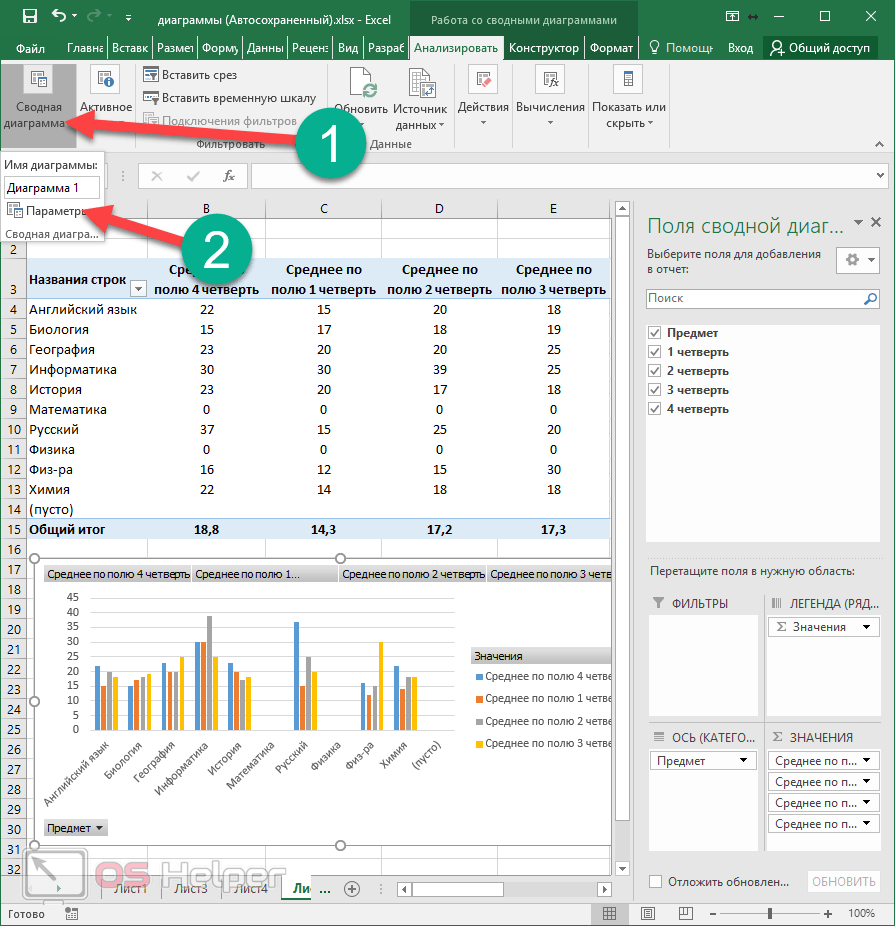
How to make a pivot chart
This tool is more complex than those described above. Previously, everything happened automatically. You only had to choose the look and the type you wanted. Everything is different here. This time you will have to do everything manually.
- Select the required cells in the table and click on the corresponding icon.

- Immediately after that, the Create PivotChart window will appear. You must specify:
- table or range of values;
- the place where the object should be placed (on a new or current sheet).
- Click on the "OK" button to continue.

- As a result, you will see:
- an empty pivot table;
- empty chart;
- pivot chart fields.

- It is necessary to move the desired fields in the area with the mouse (at your discretion):
- legends;
- values.

- In addition, you can customize what kind of value you want to display. To do this, right-click on each field and click on the "Value field parameters ..." item.

- As a result, the "Value Field Parameters" window will appear. Here you can:
- sign the source with your estate;
- select the operation to use to flatten the data in the selected field.
Click on the "OK" button to save.

Analyze Tab
After you create the PivotChart, you will have a new Analyze tab. It will disappear immediately if another object becomes active. To return, just click on the diagram again.

Let's take a closer look at each section, because with the help of them you can change all the elements beyond recognition.
Pivot table options
- Click on the very first icon.
- Select Options.
- This will bring up the settings window for this object. Here you can set the desired table name and many other parameters.

To save the settings, click on the "OK" button.
How to change the active field
If you click on this icon, you will see that all tools are inactive.

In order to be able to change any element, you need to do the following.
- Click on something in your diagram.

- As a result, this field will be highlighted with "circles".
- If you click on the Active Field icon again, you will see that the tools have become active.

- For settings, click on the appropriate field.

- As a result, the "Field parameters" window will appear.

- For additional settings, go to the Layout and Print tab.

- To save the changes made, you must click on the "OK" button.
How to insert a slice
Optionally, you can customize the selection by specific values. This feature makes it very convenient to analyze the data. Especially if the table is very large. In order to use this tool, you need to take the following steps:
- Click on the "Insert Slicer" button.
- As a result, a window will appear with a list of fields that are in the pivot table.

- Select any field and click on the "OK" button.

- As a result, a small window will appear (you can move it to any convenient place) with all the unique values (summary totals) for this table.

- If you click on any line, you will see that all other records in the table have disappeared. The only thing left is where the average corresponds to the selected one.

That is, by default (when all lines are highlighted in blue in the slicer window), all values are displayed in the table.
- If you click on another number, the result will change immediately.

- The number of lines can be absolutely any (at least one).

Both the pivot table and the diagram, which is built by its values, will change.
- If you want to delete a slice, you need to click on the cross in the upper right corner.

- This will restore the table to its original form.

In order to remove this slice window, you need to take a few simple steps:
- Right-click on this item.
- After that, a context menu will appear, in which you need to select the item "Delete‘ field name ’".

- The result will be as follows. Notice that on the right side of the editor there is again a panel for configuring the fields of the pivot table.

How to insert a timeline
In order to insert a slice by date, you need to do the following steps.
- Click on the corresponding button.

- In our case, we will see the following error window.

The fact is that for a slice by date, the table must have the corresponding values.
The principle of operation is completely identical. You will simply filter the output of records not by numbers, but by dates.
How to refresh data in a chart
To update the information in the table, click on the corresponding button.

How to change build information
To edit a range of cells in a table, you must perform the following operations:
- Click on the "Data Source" icon.
- In the menu that appears, select the item of the same name.

- Next, you will be asked to specify the required cells.
- Click on "OK" to save the changes.

Editing a chart
If you are working with a chart (it doesn't matter which one - regular or pivot), you will see the "Design" tab.

There are a lot of tools on this panel. Let's take a closer look at each of them.
Add item
If you wish, you can always add some object that is not present in this chart template. This requires:
- Click on the "Add Chart Element" icon.
- Select the desired object.

Thanks to this menu, you can change your chart and table beyond recognition.
If you don't like the standard template when creating your diagram, you can always use other layout options. To do this, it is enough to follow these steps.
- Click on the corresponding icon.
- Select the layout you want.

You don't have to make changes to your object right away. When you hover over any icon, a preview will be available.

If you find something suitable, just click on this template. The appearance will automatically change.
In order to change the color of the elements, you need to follow these steps.
- Click on the corresponding icon.
- As a result, you will see a huge palette of different shades.

- If you want to see how it will look on your diagram, just hover your cursor over any of the colors.

- To save the changes, you need to click on the selected shade.
In addition, you can use ready-made design themes. To do this, you need to do a few simple operations.
- Expand the full list of options for this tool.

- In order to see how it looks in an enlarged form, just hover the cursor over any of the icons.
- To save the changes, click on the selected option.
In addition, manipulations with the displayed information are available. For example, you can swap rows and columns.

After clicking on this button, you will see that the diagram looks completely different.
This tool is very helpful in the event that you cannot correctly specify the fields for rows and columns when building this object. If you made a mistake or the result looks ugly - click on this button. Perhaps it will become much better and more informative.

If you press it again, then everything will come back.

In order to change the range of data in the table for building a chart, you need to click on the "Select data" icon. In this window you can
- select the required cells;
- remove, change or add rows;
- edit the labels of the horizontal axis.

To save the changes, click on the "OK" button.
How to change the chart type
- Click on the indicated icon.
- In the window that appears, select the template you need.

- When you select any of the items on the left side of the screen, the options for building a diagram will appear on the right.

- For easier selection, you can hover over any of the thumbnails. As a result, you will see it at an enlarged size.

- To change the type, click on any of the options and save with the "OK" button.
Conclusion
In this article, we walked through the technology of building charts in the Excel editor step by step. In addition, special attention was paid to the design and editing of the created objects, since it is not enough to be able to use only ready-made options from Microsoft developers. You must learn to change the look to suit your needs and be original.
If you are having trouble with something, you may be highlighting the wrong element. Please note that each shape has its own unique properties. If you were able to modify something, for example, with a circle, then you will not be able to do the same with the text.
Video instruction
If for some reason nothing comes out for you, no matter how hard you try, a video is added below in which you can find various comments on the steps described above.
Subscribe to news