If your engineering background is similar to mine, then you probably know a lot about various types linear filters, the main task of which is to pass a signal in one frequency range and delay signals in other ranges. These filters are, of course, indispensable for many types of noise. However, in the real world of embedded systems, it takes a little time to realize that classical linear filters are useless against impulse noise (burst noise, popcorn noise).
Impulse noise usually arises from pseudo random events. For example, a two-way radio may switch near your device, or some static discharge may occur. Whenever this happens, the input signal may be temporarily distorted.
For example, as a result analog to digital conversion we get the following series of values: 385, 389, 912, 388, 387. The value 912 is supposedly anomalous and should be rejected. If you try to use a classic linear filter, you will notice that the value 912 will have a significant effect on the output. The best solution in this case will use the median filter.
Despite the obviousness of this approach, my experience is that median filters are remarkably rare in embedded systems. Perhaps this is due to a lack of knowledge about their existence and difficulty with implementation. I hope my post to some extent remove these obstacles.
The idea behind the median filter is simple. It selects an average from a group of input values and outputs it. And usually the group has an odd number of values, so there is no problem with the choice
Until recently, I distinguished three classes median filters, differing in the number of values used:
Filter using 3 values (smallest possible filter),
- filter using 5, 7 or 9 values (most used),
- filter using 11 or more values.
Now I stick to a simpler classification:
Filter using 3 values,
- filter using more than 3 values.
Median filter by 3
This is the smallest possible filter. It is easily implemented with a few statements and hence has a small and quick code.
uint16_t middle_of_3(uint16_t a, uint16_t b, uint16_t c)
{
uint16_t middle;
If ((a<= b) && (a <= c)){
middle = (b<= c) ? b: c;
}
else(
if ((b<= a) && (b <= c)){
middle = (a<= c) ? a: c;
}
else(
middle = (a<= b) ? a: b;
}
}
return middle;
}
Median filter > 3
For a filter size greater than 3, I suggest you use the algorithm described by Phil Ekstrom in the November 2000 issue of Embedded Systems Programming. Extrom uses a linked list. The good thing about this approach is that when the array is sorted, removing the old value and adding a new one doesn't make the array significantly cluttered. Therefore, this approach works well with large filters.
Keep in mind, there were some bugs in the original published code, which Ekstrom later fixed. Considering that it is difficult to find something on embedded.com now, I decided to publish my implementation of its code. The code was originally written in Dynamic C, but has been ported to standard C for this post. The code is supposedly working, but it's up to you to fully test it.
#define NULL 0
#define STOPPER 0 /* Smaller than any datum */
#define MEDIAN_FILTER_SIZE 5
uint16_t MedianFilter(uint16_t datum)
{
struct pair(
struct pair *point; /* Pointers forming list linked in sorted order */
uint16_tvalue; /* Values to sort */
};
/* Buffer of nwidth pairs */
static struct pair buffer = (0);
/* Pointer into circular buffer of data */
static struct pair *datpoint = buffer;
/* chain stopper */
static struct pair small = (NULL, STOPPER);
/* Pointer to head (largest) of linked list.*/
static struct pair big = (&small, 0);
/* Pointer to successor of replaced data item */
struct pair *successor;
/* Pointer used to scan down the sorted list */
struct pair *scan;
/* Previous value of scan */
struct pair *scanold;
/* Pointer to median */
struct pair *median;
uint16_t i;
if (datum == STOPPER)(
datum = STOPPER + 1; /* No stoppers allowed. */
}
If ((++datpoint - buffer) >= MEDIAN_FILTER_SIZE)(
datapoint = buffer; /* Increment and wrap data in pointer.*/
}
datapoint->value = datum; /* Copy in new datum */
successor = datepoint->point; /* Save pointer to old value"s successor */
median = /* Median initially to first in chain */
scanold = NULL; /* Scanold initially null. */
scan = /* Points to pointer to first (largest) datum in chain */
/* Handle chain-out of first item in chain as special case */
if (scan->point == datapoint)(
scan->point = successor;
}
scan = scan->point ; /* step down chain */
/* Loop through the chain, normal loop exit via break. */
for (i = 0 ; i< MEDIAN_FILTER_SIZE; ++i){
/* Handle odd-numbered item in chain */
if (scan->point == datapoint)(
scan->point = successor; /* Chain out the old datum.*/
}
If (scan->value< datum){ /* If datum is larger than scanned value,*/
datpoint->point = scanold->point; /* Chain it in here. */
scanold->point = datepoint; /* Mark it chained in. */
datum = STOPPER;
};
/* Step median pointer down chain after doing odd-numbered element */
median = median->point; /* Step median pointer. */
if (scan == &small)(
break; /* Break at the end of the chain */
}
scanold=scan; /* Save this pointer and */
scan = scan->point; /* step down chain */
/* Handle even-numbered item in chain. */
if (scan->point == datapoint)(
scan->point = successor;
}
If (scan->value< datum){
datpoint->point = scanold->point;
scanold->point = datepoint;
datum = STOPPER;
}
If (scan == &small)(
break;
}
scanold=scan;
scan = scan->point;
}
return median->value;
}
To use this filter, simply call the function each time you receive a new input value. The function will return the average value of the last accepted values, the number of which is determined by the MEDIAN_FILTER_SIZE constant.
This algorithm can use a fair amount of RAM (depending on the size of the filter, of course) because it saves input values and structure pointers. However, if this is not a problem, then the algorithm is really good to use because it is significantly faster than sort-based algorithms.
Median filtering based on sorting
In an older version of this article, for median filters of size 5, 7, or 9, I supported the sorting algorithm approach. Now I have changed my mind. However, if you would like to use them, I provide you with the basic code:
if (ADC_Buffer_Full)(
Uint_fast16_t adc_copy;
uint_fast16_t filtered_cnts;
/* Copy the data */
memcpy(adc_copy, ADC_Counts, sizeof(adc_copy));
/* Sort it */
shell_sort(adc_copy, MEDIAN_FILTER_SIZE);
/* Take the middle value */
filtered_cnts = adc_copy[(MEDIAN_FILTER_SIZE - 1U) / 2U];
/* Convert to engineering units */
...
Conclusion
The use of median filters comes with a cost. It is obvious that median filters add a delay to stepwise changing values. Also, median filters can completely overwrite the frequency information in the signal. Of course, if you are only interested in constant values, then this is not a problem.
With these reservations in mind, I still strongly recommend that you use median filters in your designs.
Recently, I had to face the need for software filtering of ADC data. Googling and smoking (various documentation) led me to two technologies: Low Pass Filter (LPF) and Median Filter. There is a very detailed article about the LPF in the Easyelectronics community, so further we will talk about the median filter.
Disclaimer (excuse): This article is for the most part a nearly verbatim translation of an article from the embeddedgurus site. However, the translator (I) also used the above algorithms in the work, found them useful, and possibly of interest to this community.
So, any linear filter is designed to pass signals in a given frequency band, and attenuate all others as much as possible. Such filters are indispensable if you want to eliminate the influence of all kinds of noise. However, in the real world of embedded systems, the designer may be faced with the fact that these classic filters are practically useless against short-term powerful spikes.
This type of noise is usually caused by some random event, such as an electrostatic discharge, an alarm key fob near the device, and so on. In this case, the input signal can take a deliberately impossible value. For example, the following data came from the ADC: 385, 389, 388, 388, 912, 388, 387. Obviously, the value 912 is false here and should be discarded. When using a classic filter, it is almost certain that this large number will affect the output value greatly. The obvious solution here is to use a median filter.
True to its name, the median filter passes the average of a set of values. Usually the size of this group is odd to avoid ambiguity in choosing the mean. The main idea is that there is a buffer with several values, from which the median is selected.
Differences between the median and the arithmetic mean
Suppose there are 19 poor people and one billionaire in one room. Everyone puts money on the table - the poor from their pocket, and the billionaire from a suitcase. Each poor person puts in $5, and each billionaire puts in $1 billion (109). The total is $1,000,000,095. If we divide the money in equal shares among 20 people, we get $50,000,004.75. This will be the arithmetic average of the amount of cash that all 20 people in that room had.
The median in this case will be equal to $5 (half the sum of the tenth and eleventh, middle values of the ranked series). It can be interpreted as follows. By dividing our company into two equal groups of 10 people, we can say that in the first group, each put no more than $5 on the table, while in the second, no less than $5. In general, we can say that the median is how much the average person brought with him. On the contrary, the arithmetic mean is an inappropriate characterization, since it greatly exceeds the amount of cash available to the average person.
en.wikipedia.org/wiki/Median_ (statistics)
By the size of this set, we divide the filters into two types:
Dimension = 3
Dimension > 3
Filter dimension 3
Dimension three is the smallest possible. It is possible to calculate the average value using only a few IF operations. Below is the code that implements this filter:uint16_t middle_of_3(uint16_t a, uint16_t b, uint16_t c) ( uint16_t middle; if ((a<= b) && (a <= c)) { middle = (b <= c) ? b: c; } else if ((b <= a) && (b <= c)) { middle = (a <= c) ? a: c; } else { middle = (a <= b) ? a: b; } return middle; }
Filter dimension >3
For a filter with dimensions greater than three, I suggest using the algorithm proposed by Phil Ekstrom in the November issue of Embedded Systems magazine, and rewritten from Dynamic C to standard C by Nigel Jones. The algorithm uses a singly linked list, and takes advantage of the fact that when an array is sorted, removing the oldest value and adding a new one does not break the sort.#define STOPPER 0 /* Smaller than any datum */ #define MEDIAN_FILTER_SIZE (13) uint16_t median_filter(uint16_t datum) ( struct pair ( struct pair *point; /* Pointers forming list linked in sorted order */ uint16_t value; /* Values to sort */ ); static struct pair buffer = (0); /* Buffer of nwidth pairs */ static struct pair *datpoint = buffer; /* Pointer into circular buffer of data */ static struct pair small = (NULL, STOPPER ); /* Chain stopper */ static struct pair big = (&small, 0); /* Pointer to head (largest) of linked list.*/ struct pair *successor; /* Pointer to successor of replaced data item */ struct pair *scan; /* Pointer used to scan down the sorted list */ struct pair *scanold; /* Previous value of scan */ struct pair *median; /* Pointer to median */ uint16_t i; if (datum == STOPPER ) ( datum = STOPPER + 1; /* No stoppers allowed. */ ) if ((++datpoint - buffer) >= MEDIAN_FILTER_SIZE) ( datpoint = buffer; /* Increment and wrap data in pointer.*/ ) datp oint->value = datum; /* Copy in new datum */ successor = datpoint->point; /* Save pointer to old value"s successor */ median = /* Median initially to first in chain */ scanold = NULL; /* Scanold initially null. */ scan = /* Points to pointer to first (largest) datum in chain */ /* Handle chain-out of first item in chain as special case */ if (scan->point == datpoint) ( scan->point = successor; ) scanold = scan; /* Save this pointer and */ scan = scan->point ; /* step down chain */ /* Loop through the chain, normal loop exit via break. */ for (i = 0 ; i< MEDIAN_FILTER_SIZE; ++i)
{
/* Handle odd-numbered item in chain */
if (scan->point == datpoint) ( scan->point = successor; /* Chain out the old datum.*/ ) if (scan->value< datum) /* If datum is larger than scanned value,*/
{
datpoint->point = scanold->point; /* Chain it in here. */scanold->point = datepoint; /* Mark it chained in. */ datum = STOPPER; ); /* Step median pointer down chain after doing odd-numbered element */ median = median->point; /* Step median pointer. */ if (scan == &small) ( break; /* Break at end of chain */ ) scanold = scan; /* Save this pointer and */ scan = scan->point; /* step down chain */ /* Handle even-numbered item in chain. */ if (scan->point == datpoint) ( scan->point = successor; ) if (scan->value< datum)
{
datpoint->point = scanold->point; scanold->point = datepoint; datum = STOPPER; ) if (scan == &small) ( break; ) scanold = scan; scan = scan->point; ) return median->value; )
To use this code, we simply call the function every time a new value appears. It will return the median of the last MEDIAN_FILTER_SIZE measurements.
This approach requires quite a lot of RAM, as You have to store both values and pointers. However, it is quite fast (58µs at 40MHz PIC18).
conclusions
Like most things in the embedded world, the Median filter comes at a price. For example, it introduces a one-read latency with continuously growing input values. In addition, this filter greatly distorts information about the frequency of the signal. Of course, if we are only interested in the constant component, this does not create any special problems.- Median filtering is non-linear, since the median of the sum of two arbitrary sequences is not equal to the sum of their medians, which in some cases can complicate the mathematical analysis of signals.
- The filter causes flattening of the vertices of triangular functions.
- Suppression of white and Gaussian noise is less effective than linear filters. Weak efficiency is also observed when fluctuation noise is filtered.
- As the filter window size increases, sharp signal changes and jumps are blurred.
The disadvantages of the method can be reduced by using median filtering with adaptive resizing of the filter window depending on the signal dynamics and the nature of the noise (adaptive median filtering). As a criterion for the size of the window, you can use, for example, the magnitude of the deviation of the values of neighboring samples relative to the central ranked sample /1i/. When this value decreases below a certain threshold, the window size increases.
16.2. MEDIAN FILTERING OF IMAGES.
Noise in images. No registration system provides perfect quality images of the studied objects. Images in the process of formation by their systems (photographic, holographic, television) are usually exposed to various random interference or noise. The fundamental problem in the field of image processing is effective removal noise while maintaining image details that are important for subsequent recognition. The complexity of solving this problem essentially depends on the nature of the noise. Unlike deterministic distortions, which are described by functional transformations of the original image, additive, impulse, and multiplicative noise models are used to describe random effects.
The most common type of interference is random additive noise, which is statistically independent of the signal. The additive noise model is used when the signal at the output of the system or at any stage of the transformation can be considered as the sum of the useful signal and some random signal. The additive noise model well describes the effect of film grain, fluctuation noise in radio engineering systems, quantization noise in analog-to-digital converters, etc.
Additive Gaussian noise is characterized by adding values with a normal distribution and zero mean to each pixel in the image. Such noise is usually introduced at the stage of formation digital imaging. The contours of objects carry the main information in images. Classical linear filters can effectively remove statistical noise, but the degree of blurring of fine details in the image may exceed the allowable values. To solve this problem, non-linear methods are used, for example, Perron and Malick anisotropic diffusion algorithms, bilateral and trilateral filters. The essence of such methods lies in the use of local estimates that are adequate for determining the contour in the image, and smoothing such areas to the least extent.
Impulse noise is characterized by the replacement of some of the pixels in the image by fixed or random variable. In the image, such interference appears as isolated contrasting dots. Impulse noise is typical for image input devices with television camera, systems for transmitting images over radio channels, as well as for digital systems transmission and storage of images. To remove impulse noise, a special class of non-linear filters built on the basis of rank statistics is used. The general idea of such filters is to detect the position of the pulse and replace it with an estimated value, while keeping the rest of the image pixels unchanged.
two-dimensional filters. Median image filtering is most effective if the image noise has an impulsive character and is a limited set of peak values against a background of zeros. As a result of applying the median filter, sloping areas and sharp changes in brightness values in the images do not change. This is very useful property specifically for images in which, as is known, the contours carry the main information.
| Rice. 16.2.1. |
With median filtering of noisy images, the degree of smoothing of object contours directly depends on the size of the filter aperture and the shape of the mask. Examples of the shape of masks with a minimum aperture are shown in Figs. 16.2.1. At small aperture sizes, the contrast details of the image are better preserved, but are suppressed to a lesser extent. impulse noise. For large apertures, the opposite is observed. Optimal choice the shape of the smoothing aperture depends on the specifics of the problem being solved and the shape of the objects. This is of particular importance for the problem of preserving differences (sharp brightness boundaries) in images.
Under the image of the difference we mean an image in which the points on one side of a certain line have the same value but, and all points on the other side of this line are the value b, b¹ a. If the filter aperture is symmetrical with respect to the origin and contains it, then the median filter preserves any image of the drop. This is done for all apertures with an odd number of samples, i.e. except for apertures ( square frames, rings) that do not contain the origin. However, square frames and rings will only slightly change the drop.
 Rice. 16.2.2. Rice. 16.2.2. |
To simplify further consideration, we restrict ourselves to an example of a filter with a square mask of size N × N, with N=3. The sliding filter scans the image samples from left to right and from top to bottom, while the input two-dimensional sequence is also represented as a sequential numerical series of samples (x(n)) from left to right from top to bottom. From this sequence, at each current point, the filter mask extracts the array w(n), as a W-element vector, which in this case contains all elements from the 3x3 window centered around x(n) and the center element itself, if provided by the mask type:
w(n) = . (16.2.1)
In this case, the x i values correspond to a left-to-right and top-to-bottom mapping of a 3×3 window into a one-dimensional vector, as shown in Fig. 16.2.2.
The elements of this vector, as well as for a one-dimensional median filter, can also be ordered in a row in ascending or descending order of their values:
r(n) = , (16.2.2)
the median value is defined y(n) = med(r(n)), and the center sample of the mask is replaced by the median value. If the mask type does not include the central sample in series 16.2.1, then the median value is the average of the two central samples of series 16.2.2.
The above expressions do not explain how the output signal is found near end and boundary points in finite sequences and images. One of simple tricks is that you need to find the median of only those points inside the image that fall within the aperture. Therefore, for points close to boundaries, medians will be determined from fewer points.
On fig. 16.2.3 shows an example of clearing a noisy image with a median Chernenko filter /2i/. The image noise over the area was 15%; for cleaning, the filter was applied successively 3 times.
  Rice. 16.1.5. Rice. 16.1.5. |
Median filtering can also be performed in a recursive variant, in which the values above and to the left of the central reference in the mask (in this case, x 1 (n) - x 4 (n) in Fig. 16.2.2) in series 16.2.1 are replaced by already values calculated in previous cycles y 1 (n)-y 4 (n).
Adaptive two-dimensional filters. The contradiction in the dependence of the degree of noise suppression and signal distortion on the filter aperture is smoothed out to some extent when filters with a dynamic mask size are used, with the aperture size adapted to the nature of the image. In adaptive filters, large apertures are used in monotonous areas of the processed signal (better noise suppression), and small apertures are used near inhomogeneities, preserving their features, while the size sliding window filter is set depending on the distribution of pixel brightness in the filter mask. They are based, as a rule, on the analysis of the brightness of the neighborhoods of the central point of the filter mask.
The simplest algorithms for dynamically changing the aperture of a filter that is symmetrical along both axes usually work according to a threshold brightness coefficient S threshold = , set on the basis of empirical data. At each current position of the mask on the image, the iterative process starts from the minimum size aperture. The deviations of the brightness of neighboring pixels A(r, n) that fall into a window of size (n x n) relative to the brightness of the central sample A(r) are calculated by the formula:
S n (r) = |A(r,n)/A(r) – 1|. (16.2.3)
The criterion according to which the mask size is increased with the central sample r and the next iteration is performed has the form:
max< S порог. (16.2.4)
The maximum mask size (number of iterations) is usually limited. For non-square masks with dimensions (n x m), iterations can be calculated with a separate increase in the parameters n and m, as well as with a change in the shape of the masks during iterations.
Filters based on rank statistics . In the last two decades, digital image processing has been actively developing not linear algorithms based on rank statistics to restore damaged images various models noise. Such algorithms make it possible to avoid additional image distortion when removing noise, as well as significantly improve the results of filters on images with a high degree of noise.
The essence of the rank statistics is usually that series 16.2.1 does not include the central sample of the filter mask, and the value m(n) is calculated from series 16.2.2. At N=3 according to fig. 16.2.2:
m(n) = (x 4 (n)+x 5 (n))/2. (16.2.5)
The calculation of the output value of the filter, which replaces the central sample, is performed according to the formula:
y(n) = a x(n) + (1-a) m(n). (16.2.6)
The value of the confidence coefficient a is associated by a certain dependence with the statistics of samples in the filter window (for example, the total variance of samples, the variance of the differences x(n)-xi (n) or m(n)-xi (n), the variance of positive and negative differences x(n )-xi (n) or m(n)-xi (n), etc.). In essence, the value of the coefficient a should specify the degree of damage to the central sample and, accordingly, the degree of borrowing for its correction values from the samples m(n). The choice of the statistical function and the nature of the dependence of the coefficient a on it can be quite diverse and depend both on the size of the filter aperture and on the nature of the images and noise.
literature
44. Bolshakov I.A., Rakoshits V.S. Applied theory of random flows, M.: Sov. radio, 1978, - 248s.
46. Huang T.S. et al. Fast algorithms in digital image processing. - M.: Radio and communication, 1984. - 224 p.
47. Soifer V.A. computer processing images. Part 2. Methods and algorithms. - Soros Educational Journal No. 3, 1996.
48. Apalkov I.V., Khryashchev V.V. Removing noise from images based on non-linear algorithms using rank statistics. - Yaroslavl State University, 2007.
1i. Yarovoy N.I. Adaptive median filtering. - http://www.controlstyle.ru/articles/science/text/amf/
2i. Chernenko S.A. median filter. - http://www.logis-pro.kiev.ua/math_power_medianfilter_ru.html.
3i. Radchenko Yu.S. Efficiency of signal reception against the background of combined interference with additional processing in the median filter. - "Journal of Radio Electronics", No. 7, 2001. / http://jre.cplire.ru/iso/jul01/2/text.html
About the noticed errors and suggestions for additions: [email protected]
Copyright ©2008 Davydov A.V.
Introduction
median filtering digital signal
digital processing signals has found wide application in various fields of activity: television, radar, communications, meteorology, seismology, medicine, speech analysis and telephony, as well as in the processing of images and fields of various nature. In some areas of economic activity, such as banking, the processing of digital financial flows is of fundamental importance.
The development of computer and microprocessor technology leads to the creation of more and more reliable, high-speed, miniature, high-quality and inexpensive equipment. Digital technologies have become so widespread that we use them in everyday life, without particularly noticing: cellular telephone, CD player, computer, etc.
In the course of this work, it is necessary to consider the advantages and disadvantages of median filtering. Learn how median filters work. Using the MatLab712 R2011a program, show its operation using an example.
Theoretical part of DSP
median filter
All linear filtering algorithms lead to smoothing of sharp changes in the brightness of images that have been processed. This shortcoming, which is especially significant if the consumer of information is a person, cannot in principle be excluded within the framework of linear processing. The point is that linear procedures are optimal for a Gaussian distribution of signals, noise, and observed data. Real images, strictly speaking, do not obey this probability distribution. Moreover, one of the main reasons for this is the presence of various borders in images, brightness differences, transitions from one texture to another, etc. Yielding to a local Gaussian description within limited areas, many real images in this regard are poorly represented as globally Gaussian objects . This is the reason for the poor transfer of boundaries in linear filtering.
The second feature of linear filtering is its optimality, as just mentioned, with the Gaussian nature of the noise. Usually, this condition is met by noise interference in images, therefore, when suppressing them, linear algorithms have high performance. However, one often has to deal with images distorted by other types of noise. One of them is impulse noise. When exposed to it, white and (and) black dots are observed on the image, randomly scattered around the frame. The use of linear filtering in this case is inefficient - each of the input pulses (essentially a delta function) gives a response in the form of a filter impulse response, and their combination contributes to the propagation of noise over the entire frame area.
A successful solution to these problems is the use of median filtering, proposed by J. Tukey in 1971 for the analysis of economic processes. The most comprehensive study of median filtering as applied to image processing is presented in the collection. Note that median filtering is a heuristic processing method, its algorithm is not mathematical solution strictly formulated problem. Therefore, researchers pay great attention to the analysis of the efficiency of image processing based on it and comparison with other methods.
When applying the median filter (MF), each point of the frame is sequentially processed, resulting in a sequence of estimates. Conceptually, the processing at different points is independent (in this way, the MF is similar to a mask filter), but in order to speed it up, it is advisable to algorithmically use previously performed calculations at each step.
Median filtering uses a two-dimensional window (filter aperture), which usually has central symmetry, with its center located at the current filtering point. On fig. 1.1 shows two examples of the most commonly used window options in the form of a cross and in the form of a square. Aperture sizes are among the parameters that are optimized in the process of analyzing the effectiveness of the algorithm. The image samples that are within the window form the working sample of the current step.

Rice. 1.1.
The two-dimensional nature of the window allows for essentially two-dimensional filtering, since data from both the current row and column, as well as from neighboring ones, are used to form an estimate. Denote the working sample as a one-dimensional array; the number of its elements is equal to the size of the window, and their arrangement is arbitrary. Usually, windows with an odd number of points are used (this is automatically ensured if the aperture is centrally symmetric and if the central point itself enters into its composition). If you sort a sequence in ascending order, then its median will be the sample element that occupies a central position in this ordered sequence. The number thus obtained is the filtering product for the current point of the frame. It is clear that the result of such processing does not really depend on the sequence in which image elements are presented in the working sample. Let us introduce the formal notation of the described procedure in the form:
x * =med(y 1 , y 2 ,…, y n) (1.1)
Consider an example. Suppose that the selection has the form: Y=(136,110,99,45,250,55,158,104,75), and the element 250, located in its center, corresponds to the current filtering point (i 1 , i 2) (Fig. 1.1). Great importance brightness at this point in the frame may be the result of impulse (dot) interference. The sample ordered in ascending order has the form (45,55,75,99,104,110,136,158,250), therefore, in accordance with the procedure (1.1), we obtain x * =med(y 1 , y 2 ,…, y 9)=104. We see that the influence of “neighbors” on the result of filtering at the current point led to the “ignoring” of the impulse burst of brightness, which should be considered as a filtering effect. If the impulse noise is not point, but covers some local area, then it can also be suppressed. This will happen if the size of this local area is less than half the size of the MF aperture. Therefore, to suppress impulse noise that affects local areas of the image, it is necessary to increase the size of the MF aperture.
From (1.1) it follows that the action of the MF consists in “ignoring” the extreme values of the input sample, both positive and negative outliers. This principle of interference suppression can also be applied to reduce noise in the image. However, a study of noise suppression using median filtering shows that its effectiveness in solving this problem is lower than that of linear filtering.
The experimental results illustrating the operation of the MF are shown in Figs. 1.2. In the experiments, an MF was used, which has a square aperture with a side equal to 3. The left row shows images distorted by interference, and the right row shows the results of their median filtering. On fig. 1.2 a and fig. 1.2.c shows the original image distorted by impulse noise. When it was superimposed, a random number generator was used with a uniform distribution law over the interval, which generates independent random numbers at all points of the frame. The noise intensity was set by the probability p of its occurrence at each point. If for a random number n i1i2 formed at the point (i 1 , i 2) the condition n i1i2 Rice. 1.2. Rice. 1.2. e shows an image distorted by independent Gaussian noise at a signal-to-noise ratio q 2 =-5 dB, and fig. 1.2.e - the result of its filtering by the median filter. The conditions of this experiment make it possible to compare its results with the results of the linear filtering considered above. Table 1.1 provides data to enable such a comparison. For various filtering methods, this table gives the values of the relative mean square errors q 2 and the noise attenuation coefficient r for the case when the signal-to-noise ratio at the filter input is -5 dB. Table 1.1. Comparison of noise suppression efficiency in image filtering, q 2 =-5 dB. The two-dimensional Wiener filter has the highest efficiency, reducing the mean square of errors by a factor of 17. The median filter has the lowest efficiency among all considered filters, it corresponds to r = 5.86. However, this number indicates that even with its help it is possible to significantly reduce the level of noise in the image. However, as mentioned above, and as shown in Fig. 1.2.e, median filtering smoothes the edges of the image to a lesser extent than any linear filtering. The mechanism of this phenomenon is very simple and consists in the following. Let us assume that the filter aperture is located near the border separating the light and dark areas of the image, while its center is located in the dark area. Then, most likely, the working sample will contain a larger number of elements with low brightness values, and, therefore, the median will be among those elements of the working sample that correspond to this area of the image. The situation is reversed if the center of the aperture is shifted to a region of higher brightness. But this means that the MF is sensitive to changes in brightness. There are a huge number of interpretations of the methods of MF operation, let's consider another one, using it as an example when processing images of blood cells - granulocytes. Before measuring the size of a granulocyte, its image was subjected to smoothing with a median filter in order to eliminate granules that could affect the measurement result. Usually, in the process of median filtering, the signal values in a certain neighborhood of the point where the filter response is calculated are sorted in ascending or descending order in a variational series. The filter response is defined as the median -- the signal value of the middle (center) of the variation series. In what follows, this neighborhood will be referred to as the filter window. In addition, for simplicity, we will consider a filter with a square window of size n×n . Therefore, when calculating the median in the filter window, the number of data operations, such as the number of sort operations, is n 2 . When processing an image with a size of M?N dots (pixels), the number of data operations will be large and will be M?N?n 2 . Different operations require different execution times. By sequentially scanning an image, the most time-consuming sorting operations can be reduced. Thus, when passing from point o1 with window w1 to point o2 with window w2 in Fig. 1.3. it is possible to exclude the points of column 1 from the variation row of window w1, sort the points of column 6 and merge the two resulting variation rows into one. Such an algorithm works faster than independent sorting in each window, but the total number of data manipulations (albeit less laborious), for example, at least sorting through the data, remains the same, i.e., quite large. Therefore, median filtering of images is usually limited to windows of 3×3 or 5×5 and rarely larger, which is quite sufficient, for example, to eliminate impulse noise. Rice. 1.3. Scanning an Image with a Median Filter Window
The same restrictions are forcibly accepted for various non-linear operations of morphological processing performed in the geometric space of the image, and which, unlike linear operations, cannot be performed in Fourier space. However, there are a number of image processing problems that could be efficiently solved using a median filter, but they require a large window size. One of these tasks will be discussed below. Therefore, a possible increase in the speed of median filtering promises great prospects in image processing problems. Median filtering methods are quite diverse. They can be improved. One such upgrade is called adaptive median filtering. Median filtering also has its drawbacks. In particular, it has been experimentally established that this method has a relatively low efficiency in filtering the so-called fluctuation noise. In addition, when the mask size is increased, the contours of the image are blurred and, as a result, the clarity of the image is reduced. These disadvantages of the method can be minimized by using median filtering with a dynamic mask size (adaptive median filtering). The principle of calculating the central reference for local image processing by a sliding window remains the same. This median is from a set of ordered samples that fall into the window (mask), and the size of the sliding window (mask) is dynamic and depends on the brightness of neighboring pixels. Let us introduce the threshold coefficient of brightness deviation S threshold = . The values of the deviation of the brightness of neighboring pixels A(r, n, m), which fell into a window of size n?m, relative to the brightness of the central sample A(r) will be written in the form (1.2): Then the criterion according to which it is necessary to increase the size of the mask with a central reading r will look like this: Based on the described algorithm, a computer program was developed that confirmed in practice the advantages of adaptive median filtering. 1 IN SCIENTIFIC INSTRUMENTATION, 011, volume 1, 3, c DATA PROCESSING AND REPRESENTATION UDC: BV Bardin FAST MEDIAN FILTERING ALGORITHM A fast median filtering algorithm is proposed that uses the determination of the data median in the filter window by analyzing a local histogram. As you move from point to point as you scan an image, adjusting the histogram requires a small number of simple steps. The proposed algorithm significantly speeds up median filtering compared to traditional algorithms. This allows you to expand the scope of median filtering. Cl. words: median filtering, digital images INTRODUCTION Median filtering is a convenient tool for processing information, especially two-dimensional image information. The median filter removes fragments from the signal with sizes smaller than half the size of the filter window, and at the same time slightly or almost does not distort the rest of the signal sections. For example, a one-dimensional monotonic signal is not distorted at all by the median filter. The most well-known application of median filtering is the elimination of short impulse noise from the signal [, 3]. Moreover, the noise amplitude does not affect the result of median filtering, in contrast to the response of a linear filter. The paper shows the use of a median filter in the processing of images of blood cells and granulocytes. Here, before measuring the size of the granulocyte, its image was subjected to smoothing with a median filter in order to eliminate granules that could affect the measurement result. Usually, in the process of median filtering, the signal values in a certain neighborhood of the point where the filter response is calculated are sorted in ascending or descending order in a variational series. The filter response is defined as the median signal value of the middle (center) of the variation series. In what follows, this neighborhood will be referred to as the filter window. In addition, for simplicity, we will consider a filter with a square window of size n n. Therefore, when calculating the median in the filter window, the number of operations on the data, such as the number of sort operations, is n. When processing an image of size M N dots (pixels), the number of data operations will be large and will be M N n. Different operations require different execution times. By sequentially scanning an image, the most time-consuming sorting operations can be reduced. So, when passing from point o1 with window 1 to point o with window in Fig. 1 it is possible to exclude the points of column 1 from the variation row of window 1, sort the points of column 6 and merge the two resulting variation rows into one. Such an algorithm is faster than independent sorting in each window, however, the total number of data manipulations (albeit less laborious), for example, at least sorting through the data, remains the same, i.e., quite large. Therefore, median filtering of images is usually limited to windows 3 3 or 5 5 and rarely. 1. Scanning an image with a median filter window 135 2 136 BV BARDIN more, which is quite enough, for example, to eliminate impulse noise. The same restrictions are forcibly accepted for various non-linear operations of morphological processing performed in the geometric space of the image, and which, unlike linear operations, cannot be performed in Fourier space. However, there are a number of image processing problems that could be efficiently solved using a median filter, but they require a large window size. One of these tasks will be discussed below. Therefore, a possible increase in the speed of median filtering promises great prospects in image processing problems. FAST MEDIAN FILTERING In the paper, when considering rank image processing algorithms, it is shown that any r-th order statistics v (r) of an image element can be found from the local histogram h (q) of the distribution of neighborhood element values (windows in Fig. 1) by solving the equation v (r) h (q) r. (1) q 0 Here q = 0, 1,Q 1 is the quantum (bin) number of the histogram; v = q v quantized value of the video signal; r = 0, 1, 1 element rank: its number in the variation series; the number of elements of the neighborhood (window), or the area of the window in pixels; in our case n. The median filter is a special case of the rank filter with the response rank r = (1)/. Since Q 1 h (q), () q 0, it follows from (1) that the median q = v (r) divides the area of the histogram in half (minus the bin corresponding to q). On fig. a split histogram is shown. Here h(q) is the area of the bin corresponding to h(q). The remaining designations are clear from the figure. In this case, the following relations are valid:, (3) (1) /, (4) (1) /. (5) It is assumed to be odd. The inequality signs in the last two expressions can take place only at 1. When scanning the median filter window along the line, when moving from the point o1 to the point o in Fig. 1 histogram correction is performed as follows. 1. The data corresponding to the points of column 1 are removed from the histogram. At the same time, for each point, 1 is subtracted from the area of the corresponding bin. The data corresponding to the points of column 6 are added to the histogram. items 1 and simultaneously change the values, and. 4. Based on expressions (3), (4) and (5), the values, and q are corrected. Below is a fragment of a C program that implements the described correction algorithm. Here, in order to comply with the syntax of the C language, the subscripts at and q are replaced by lowercase letters, and the subscripts at h and v are omitted. For the case in Fig. 1 n=5 and j=1. SCIENTIFIC INSTRUMENT MAKING, 011, volume 1, 3 3 FAST MEDIAN FILTERING ALGORITHM 137 fr(i=0; i If the background value significantly differs (or changes) in the image area, then the linear filter perceives this difference as a signal jump and tries to smooth it out. This is a well-known phenomenon of edge effects. Exist various ways to deal with edge effects. Most often, this is either discarding a part of the image affected by edge effects, with a corresponding loss of some useful information, or expanding the frame with additional fields filled in such a way that there would be no jumps at the edges of the original image field containing useful information. However, there are images in the processing of which it is either impossible or very difficult to implement such approaches. So, in fig. 3 shows a microchip well with objects of PCR analysis and a signal profile according to horizontal line on the image. On fig. Figure 4 shows the calculation of the background component using linear filtering, which, as can be seen from the figure, gives large edge distortion along the well contour. The cutting of image areas distorted by edge effects is unacceptable in this case due to the large loss of useful information, and the expansion working area difficult due to the fact that this area is round, and also due to the large non-uniformity of the background along the contour of the area. On fig. 5 shows the calculation of the background using the median filter. It can be seen from the figure that the edge effects in this case are very small, but this required the use of a filter with a large pixel window or 1681 pixels per window. The image size was pixels. The median filtering time was measured on a computer with modest capabilities. He included single core processor Pentiu 4 CPU.4 Gz and RAM 51 MB. The filtering time by the traditional median filter using data sorting in the window was 33 s. The same filtration time using the proposed in present work algorithm was 0.37 s, i.e., almost two orders of magnitude less than when using traditional algorithms. It should be noted that, on the one hand, in the problem under consideration (PCR analysis), the time of 0.37 s is quite acceptable, and on the other hand, in systems using digital image processing, as a rule, much more powerful computers. Thus, the application of the proposed algorithm can significantly speed up the operation of the median filter, which, in addition, allows expanding the scope of median filtering. Rice. 4. Background calculation line filter Rice. 5. Calculation of the background by the median filter 5 FAST MEDIAN FILTERING ALGORITHM 139 REFERENCES 1. Bardin B.V. Investigation of the possibilities of median filtering in the digital processing of images of sets of local biological objects // Scientific instrumentation vol. 1,. S Gonzalez R., Woods R. Digital Image Processing. Per. from English. Moscow: Technosfera, p. 3. Yaroslavsky L.P. Digital signal processing in optics and holography. M.: Radio and communications, p. 4. Bardin B.V., Chubinsky-Nadezhdin I.V. Detection of local objects on digital microscopic images. Nauchnoe priborostroenie V. 19, 4. Bardin B.V., Manoilov V.V., Chubinskiy-Nadezhdin I.V., Vasilieva E.K., Zarutskiy I.V. Determining the size of local image objects for their identification // Scientific Instrumentation V. 0, 3. C Institute for Analytical Instrumentation RAS, St. Petersburg Contacts: Bardin Boris Vasilievich f RA, aint Petersburg Fast algrith f edian filtering using data edian deterinatin in filter ind by eans f lcal histgra analysis has been suggested. When ving fr pixel t pixel in the prcess f iage scanning crrectin f histgra requires sall nuber f nn-cplex peratins. The suggested algrith increases cnsiderably the edian filtering prcess cpared t the traditinal algriths. This enables edian filtering applicatin sphere extending. Keyrds: edian filtering, digital iaging Original layout prepared by Belenkov V.D. License ID 0980 dated October 06, 000 Signed for publication d. Format Offset paper. Offset printing. Conv. oven l Uch.-ed. l Circulation 100 copies. Type. zak. 70. С 96 St. Petersburg publishing company "Nauka" RAS, St. Petersburg, Mendeleevskaya line, 1 E-ail: Internet:.naukaspb.spb.ru First Academic Printing House "Nauka", St. Petersburg, 9 line, 1 NONLINEAR GEOMETRIC MEAN FILTER WITH EXPONENTIAL WEIGHTS Tolstunov Vladimir Andreevich Ph.D. tech. Sciences, Associate Professor, Kemerovo State University, Russian Federation, Kemerovo E-mail: [email protected] UDC 61.397 Frequency and spatial methods digital filtering Images # 05, May 01 Cherny S.A. Student, Department of Radioelectronic Systems and Devices Supervisor: Akhiyarov V.V., Candidate Efficient Modification of the Algorithm for Adaptive Median Filtering of Digital Images Yaikov Rafael Ravilevich Yaroslavl State University. P. G. Demidova 2015 What are the noises? additive Section 6. Digital processing of signals and images 377 E.E. Plakhova, E.V. Merkulova Donetsk National Technical University, Donetsk Department automated systems Open Information and Computer Integrated Technologies 64, 014 UDC 004.8/004.93/681.513.8;681.514 L. S. Kostenko Methods and algorithms for image background smoothing in pattern recognition systems UDC 519.6 + 004.4 FILTRATION OF X-RAY TOMOGRAMS BY ADAPTATION OF FILTER WINDOW SIZE TO LOCAL IMAGE CHARACTERISTICS E.N. Simonov, V.V. Laskov An algorithm for image filtering is proposed ISSN 0868 5886, p. 96 102 PROCESSING AND ANALYSIS OF SIGNALS UDC 621.391.837: 681.3 BV Bardin, IV Chubinskii-Nadezhdin DETECTION OF LOCAL OBJECTS IN DIGITAL MICROSCOPIC IMAGES Considered ICONICS IMAGE SCIENCE UDC 004.932.4 METHOD OF INTERCHANNEL COMPENSATION OF PULSED INTERFERENCE IN THE TASKS OF RECOVERY OF MULTI-COMPONENT DIGITAL IMAGES 2013 E. A. Samoilin, Dr. Tech. sciences; IN. Implementation of some image processing algorithms using CUDA technology on graphics devices N.N. Theological Tomsk State University of Digital Image Processing in UDC 621.391 A. V. IVASHKO, Ph.D. tech. sciences, prof. NTU "KhPI"; KN Yatsenko, student of NTU "KhPI" IMPLEMENTATION OF MEDIAN AND QUASI-MEDIAN FILTERS ON DIGITAL SIGNAL PROCESSORS Processing of digital images of glass microspheres by filtering and segmentation methods 77-30569/403867 # 03, March 2012 Strugailo V. V. UDC 004.932 Russia, Moscow Automobile and Road State VA Tolstunov Nonlinear filtering based on power transform 7 UDC 00467 VA Tolstunov Nonlinear filtering based on power transform A digital smoothing filter algorithm is proposed. Table of contents 6. Processing and quantitative analysis SPM images Contents 6. PROCESSING AND QUANTITATIVE ANALYSIS OF SPM IMAGES... 6-1 6.1. PURPOSE OF THE WORK... 6-2 6.2. CONTENT OF WORK... 6-2 6.3. THE TASK... Bandpass Filtering 1 Bandpass Filtering In the previous sections, filtering of fast signal variations (smoothing) and slow signal variations (detrending) was considered. Sometimes you need to highlight UDC 004.932 V.K. Zlobin, B.V. Kostrov, V.A. Sablina ALGORITHM FOR SEQUENT FILTERING OF GROUP NOISE IN IMAGE The problems of using sequence analysis methods in relation to digital Math-Net.Ru All-Russian Mathematical Portal AV Grokhovskoi, AS Makarov, Image pre-processing algorithm for vision systems, Matem. modeling and edges. tasks, 2009, UDC 61.865.8 METHODS OF INCREASING THE CONTRAST OF Raster IMAGES FOR DIGITAL VIDEO PROCESSING SYSTEMS MB Sergeev, Dr. Tech. Sciences, Professor N. V. Solovyov, Ph.D. tech. Sciences, Associate Professor A.I. The influence of filters on the classification of fingerprinting # 01, January 2015 Deon A. F., Lomov D. S. UDC: 681.3.06(075) Russia, MSTU im. N.E. Bauman [email protected] Fingerprint classes In traditional fingerprinting ISSN 0868 5886, p. 9 13 MEASUREMENT METHODS UDC 543.426; 543.9 Yu. V. Belov, I. A. Leontiev, A. I. Petrov, V. E. Kurochkin BASELINE CORRECTION OF GENETIC ANALYZER FLUORESCENT DETECTOR SIGNALS Ñóäîñòðîåíèå ñóäîðåìîíò è ýêñïëóàòàöèÿ ôëîòà UDC 004.93.4: 551.463.1 GA Popov DA Khryashchev ÎÁ ÎÄÍÎÌ ÌÅÒÎÄÅ ÍÈÇÊÎ ÀÑÒÎÒÍÎÉ ÔÈËÜÒÐÀÖÈÈ ÃÈÄÐÎËÎÊÀÖÈÎÍÍÛÕ ÈÇÎÁÐÀÆÅÍÈÉ Introduction Many recent studies Homework. Processing the results of observations of a two-dimensional random vector.1. The content and order of the work Handbook for students of institutions of general secondary education, 5th edition, corrected by Mozyr "Belyi Veter" 2 0 1 4 BURYAK R e c e n SWorld 218-27 December 2012 http://www.sworld.com.ua/index.php/ru/conference/the-content-of-conferences/archives-of-individual-conferences/december- 2012 MODERN PROBLEMS AND WAYS OF THEIR SOLUTION IN SCIENCE, FEDERAL RAILWAY TRANSPORT AGENCY educational institution higher vocational education PETERSBURG STATE UNIVERSITY OF TRACKS UDC 004.021 1 E. V. Leontieva, E. V. Medvedeva METHOD FOR RECOVERY OF RGB-COMPONENT IMAGES DISTORTED BY APPLICATIVE NOISES Ministry of Education of the Russian Federation Volgograd State Technical University Department of Materials Science and Composite Materials One-Dimensional Search Methods Guidelines Computer graphics Noise suppression and elimination Image noise reduction Image noise suppression and elimination Causes of noise: Imperfection of measurement instruments Chair software ACS G.A. SHEININA Structures and data processing algorithms Recommended by the editorial and publishing council of the university as guidelines for students of the specialty MINISTRY OF EDUCATION AND SCIENCE OF THE RUSSIAN FEDERATION STATE EDUCATIONAL INSTITUTION OF HIGHER PROFESSIONAL EDUCATION "SAMARA STATE AEROSPACE UNIVERSITY named after Academician S.P.KOROLEV" Nonlinear filtering of noisy interference fringes 245 NONLINEAR FILTERING OF NOISY INTERFERENCE FIBERS WITH A SPATIALLY DEPENDENT IMPULSAL RESPONSE OF THE SYSTEM M.V. Volkov Scientific Supervisor MINISTRY OF GENERAL AND VOCATIONAL EDUCATION OF THE RUSSIAN FEDERATION Nizhny Novgorod State University. N. I. LOBACHEVSKY Faculty of Computational Mathematics and Cybernetics Department of Mathematical STATE EDUCATIONAL INSTITUTION OF HIGHER PROFESSIONAL EDUCATION "VORONEZH STATE PEDAGOGICAL UNIVERSITY" INTRODUCTION TO ANALYSIS AND DIFFERENTIAL CALCULATION OF FUNCTIONS OF ONE VARIABLE ALGORITHMS FOR SEARCHING DISTANCES TO OBJECT PIXELS IN BINARY IMAGES Kazansky, V.V. Myasnikov, R.V. Khmelev Institute of Image Processing Systems RAS Problem statement One of the most important tasks 00 BULLETIN OF NOVGOROD STATE UNIVERSITY 55 UDC 598765 OUTLINE OF THE IMAGE OF A MOVING OBJECT information systems NovSU, [email protected] ISSN2221-2574 Television systems, transmission and image processing UDC 621.396 Construction of a test image model SN Zhiganov, IV Gashin. The paper considers a technique for constructing an image model, Control Systems and Modeling Algorithm for Robust Stability Analysis of Discrete Control Systems with Periodic Constraints MV MOROZOV Abstract. For discrete linear non-stationary systems UDC 681.5:004.93 Yu.V. Kalinichenko ON THE QUESTION OF BORDER DETECTION BY THE KENNY DETECTOR Luhansk Taras Shevchenko National University The issue of border detection by the Kenny detector is considered. Algorithm implemented Regional scientific and practical conference educational and research work of students in grades 6-11 "Applied and fundamental questions of mathematics" Applied questions of mathematics Character recognition on electronic ALGORITHMS FOR CONTROL OF THE COORDINATES OF THE RADIATION SOURCE ON THE PHOTO-SENSITIVE SURFACE OF THE MATRIX Digital Signal Processing 4/28 UDC 68.58 ADAPTIVE FILTERING OF IMAGES WITH STRUCTURAL DISTORTIONS Kostrov BV, Sablina VA. Introduction The process of registration of aerospace images is accompanied by 370 Section 6. Digital signal and image processing UDC 004. 93"12 I.S. Lichkanenko, V.N. Pchelkin Donetsk National Technical University, Donetsk Department computer systems MONITORING METHODS SPACE IMAGE PROCESSING BASED ON FREQUENCY REPRESENTATIONS A.Yu. Likhosherstny Belgorod State University e-mail: [email protected] The work presents new method filtration ISSN 1995-55. Vestnik RGRTU. 1 (issue 31). Ryazan, 0 UDC 1.391 Yu.M. Korshunov QUALITY EVALUATION OF DIGITAL FILTERS ON THE BASIS OF AN ARTIFICIALLY CREATED SIMULATION MODEL OF SIGNAL AND INTERFERENCE A method is proposed ANALYSIS OF THE DISPERSIVE COMPOSITION OF MICROSCOPIC OBJECTS WITH THE USE OF A COMPUTER Korolev D. V., Suvorov K. A. St. Petersburg State Technological Institute (Technical University), [email protected] UDC 528.854 Kuzmin S. A. STUDY OF ALGORITHMS FOR REMOVING PULSED INTERFERENCE IN VIDEO SEQUENCES The problem of improving the characteristics of object detection algorithms in video sequences by suppressing UDC 681.3.082.5 G.N. Glukhov Algorithm for digital surface smoothing An algorithm for optimal surface smoothing is proposed. The optimality criterion is the minimum of weighted sums: sums of squares Manual for students of institutions of general secondary education Compiled by G. I. Struk 5th edition Mozyr "White Wind" 2 0 1 4 UDC 372.851.046.14 LBC 74.262.21 T36 Reviewers: Candidate SWorld 8-29 June 203 http://www.sworld.com.ua/index.php/ru/conference/the-content-of-conferences/archives-of-individual-conferences/june-203 THEIR SOLUTION IN SCIENCE, TRANSPORT, Ministry of Education of the Russian Federation St. Petersburg State University of Low-Temperature and Food Technologies Department of Theoretical Mechanics STUDY OF THE REACTION FORCES OF COMPOSITE SUPPORTS UDC 004.932.72; 681.3 N. Yu. Ryazanova and V. A. Ul'ikhin ISSUES OF IMAGE SCALE WITH CONSIDERATION OF THEIR CONTENT Consideration is given to the choice of algorithms for plot detection and significance determination. UDC 621.397:621.396.96 STRAIGHT EDGING IN NOISY IMAGES V. Yu. Volkov, Dr. Tech. Sciences, Professor St. Petersburg State University of Telecommunications. prof. M. Ministry of Education and Science of the Russian Federation Altai State University O. Yu. Voronkova, S. V. Ganzha ORGANIZATIONAL AND ECONOMIC MECHANISM OF REGULATION OF LAND AND MORTGAGE RELATIONS IN MARKET CONDITIONS IMAGE RECOVERY USING NONLINEAR FILTERS OBTAINED BY IDENTIFICATION OF A LINEAR MODEL IN PARAMETERS Fursov, D.A. Elkin Academician Samara State Aerospace University ISSN 0868 5886, p. 101 106 INSTRUMENTS, INSTALLATIONS, METHODS UDC 621.38 BS Gurevich, SB Gurevich, VV Manoilov WAVELET FILTRATION OF SPATIAL FREQUENCIES DURING DISCRETIZATION OF LIGHT FIELDS Electronic journal"Proceedings of MAI". Issue 50.mai.ru/science/trud/ UDC 004.9 LBC 3.97 Technique for filtering periodic noise in digital images V.Yu. Gusev A.V. Krapivenko Abstract The article considers MODEL OF THE VISUAL SYSTEM OF A HUMAN OPERATOR IN OBJECT IMAGE RECOGNITION Yu.S. Gulina, V.Ya. Kolyuchkin Lomonosov Moscow State Technical University N.E. Bauman, The mathematical OPTO-ELECTRONIC METHODS OF CONTROL OF THE EMISSION COORDINATES ON THE MATRIX SURFACE WITH THE USE OF CENTROIDAL ALGORITHMS VI Zamyatin VV Zamyatin Altai State Technical University. UDC 621.396 REDUCING THE INFLUENCE OF 8-BIT GRAD QUANTIZATION ON THE POSSIBILITIES OF RECOVERY A. Yu. V.A. Kotelnikova Lab 3 Task You are required to implement a program that performs operations on arrays. Part 1 allows the use of statically sized arrays. When doing part 2 A technique for a priori estimation of the efficiency of digital image compression in the system operational transmission data remote sensing Lands 2.3. Analysis of compression algorithms for linearity Lesson 3 REGRESSION ANALYSIS FOR PROCESSING EXPERIMENTAL RESULTS Regression analysis is often used in chemistry to process experimental data, the totality of which is represented by some Workshop for students of institutions of general secondary education Mozyr "White Wind" 2 0 1 4 Federal Agency for Education State Educational Institution of Higher Professional Education Don State Technical University Department of Computer Science MINISTRY OF EDUCATION AND SCIENCE OF THE RUSSIAN FEDERATION Federal State Budgetary Educational Institution of Higher Professional Education "NATIONAL RESEARCH TOMSK POLYTECHNICAL MINISTRY OF HEALTH OF THE REPUBLIC OF BELARUS METHOD OF DIFFERENTIAL DIAGNOSIS OF CHRONIC PANCREATITIS AND PANCREAS ADENOCARCINOMA PHASE RECOVERY OF INTERFERENCE STRIPS BY THE METHOD OF NONLINEAR TWO-DIMENSIONAL KALMAN FILTRATION Zakharov The characteristics of a two-dimensional discrete nonlinear Kalman filter under dynamic estimation are studied. COLLECTION OF SCIENTIFIC WORKS OF NSTU. 28.4(54). 37 44 UDC 59.24 ON THE COMPLEX OF PROGRAMS FOR SOLVING THE PROBLEM OF IDENTIFICATION OF LINEAR DYNAMIC DISCRETE STATIONARY OBJECTS G.V. TROSHINA A set of programs was considered Proceedings of the V International Scientific and Technical School-Conference, November 3, 8 MOSCOW YOUNG SCIENTISTS 8, part 4 MIREA QUALITY ASSESSMENT OF INTERPOLATION FILTERS IN VIDEO CODING STANDARDS 8 D.B. POLYAKOV


![]()
transcript