The solution of any problem for the calculation of an electrical circuit should begin with the choice of the method by which the calculations will be made. As a rule, one and the same problem can be solved by several methods. The result in any case will be the same, and the complexity of the calculations may differ significantly. For the correct choice of the calculation method, you must first determine which class the given electrical circuit belongs to: simple electrical circuits or complex ones.
To simple include electrical circuits that contain either one source of electrical energy, or several located in the same branch of the electrical circuit. Below are two diagrams of simple electrical circuits. The first circuit contains a single voltage source, in which case the electrical circuit is clearly a simple circuit. The second contains already two sources, but they are in the same branch, therefore it is also a simple electrical circuit.
The calculation of simple electrical circuits is usually carried out in the following sequence:

The described technique is applicable to the calculation of any simple electrical circuits, typical examples are given in example No. 4 and in example No. 5. Sometimes calculations by this method can be quite voluminous and lengthy. Therefore, after finding a solution, it would be useful to check the correctness of manual calculations using specialized programs or drawing up a power balance. The calculation of a simple electrical circuit in combination with the preparation of a power balance is shown in example No. 6.
Complex electrical circuits
To complex electrical circuits include circuits containing several sources of electrical energy included in different branches. The figure below shows examples of such circuits. 
For complex electrical circuits, the method for calculating simple electrical circuits is not applicable. Simplification of circuits is impossible, because it is impossible to select a circuit section with a series or parallel connection of the same type of elements on the diagram. Sometimes, the transformation of the circuit with its subsequent calculation is still possible, but this is rather an exception to the general rule.
For the complete calculation of complex electrical circuits, the following methods are usually used:
- Application of Kirchhoff's laws (universal method, complex calculations of a system of linear equations).
- Loop current method (universal method, calculations are slightly simpler than in paragraph 1)
- Nodal stress method (universal method, calculations are slightly simpler than in paragraph 1)
- Superposition principle (universal method, simple calculations)
- Equivalent source method (useful when it is necessary to make not a complete calculation of the electrical circuit, but to find the current in one of the branches).
- Circuit equivalent transformation method (rarely applicable, simple calculations).
Features of the application of each method for calculating complex electrical circuits are described in more detail in the relevant subsections.
The essence of the calculations is, as a rule, to determine the currents in all branches and voltages on all elements (resistances) of the circuit using the known values of all circuit resistances and source parameters (EMF or current).
Various methods can be used to calculate DC electrical circuits. Among them, the main ones are:
– a method based on the compilation of the Kirchhoff equations;
– method of equivalent transformations;
– method of loop currents;
– overlay method;
– method of nodal potentials;
– equivalent source method;
The method based on the compilation of the Kirchhoff equations is universal and can be used for both single-loop and multi-loop circuits. In this case, the number of equations compiled according to the second Kirchhoff law must be equal to the number of internal circuits of the circuit.
The number of equations compiled according to the first Kirchhoff law must be one less than the number of nodes in the circuit.
For example, for this scheme
2 equations are compiled according to the 1st Kirchhoff law and 3 equations according to the 2nd Kirchhoff law.
Consider other methods for calculating electrical circuits:
The method of equivalent transformations is used to simplify circuits and calculations of electrical circuits. An equivalent conversion is understood as such a replacement of one circuit by another, in which the electrical quantities of the circuit as a whole do not change (voltage, current, power consumption remain unchanged).
Let us consider some types of equivalent circuit transformations.
a). serial connection of elements
The total resistance of series-connected elements is equal to the sum of the resistances of these elements.
R e =Σ R j (3.12)
R E \u003d R 1 + R 2 + R 3
b). parallel connection of elements.
Consider two elements R1 and R 2 connected in parallel. The voltage on these elements are equal, because. they are connected to the same nodes a and b.
U R1 = U R2 = U AB
Applying Ohm's law, we get
U R1 =I 1 R 1 ; U R2 \u003d I 2 R 2
I 1 R 1 \u003d I 2 R 2 or I 1 / I 2 \u003d R 2 / R 1
Let's apply Kirchhoff's 1st law to node (a)
I - I 1 - I 2 \u003d 0 or I \u003d I 1 + I 2
We express the currents I 1 and I 2 in terms of voltages, we get
I 1 \u003d U R1 / R 1; I 2 = U R2 / R 2
I \u003d U AB / R 1 + U AB / R 2 \u003d U AB (1 / R 1 +1 / R 2)
In accordance with Ohm's law, we have I=U AB / R E; where R e is the equivalent resistance
Considering this, one can write
U AB / R E \u003d U AB (1 / R 1 +1 / R 2),
1 / R E \u003d (1 / R 1 + 1 / R 2)
Let's introduce the notation: 1/R e =G e - equivalent conductivity
1 / R 1 \u003d G 1 - conductivity of the 1st element
1 / R 2 \u003d G 2 - conductivity of the 2nd element.
We write equation (6) in the form
G E \u003d G 1 + G 2 (3.13)
It follows from this expression that the equivalent conductivity of parallel-connected elements is equal to the sum of the conductivities of these elements.
Based on (3.13), we obtain the equivalent resistance
R E \u003d R 1 R 2 / (R 1 + R 2) (3.14)
in). Transformation of the triangle of resistances into an equivalent star and inverse transformation.
The connection of three elements of the chain R 1, R 2, R 3, which has the form of a three-beam star with a common point (node), is called a “star” connection, and the connection of the same elements, in which they form the sides of a closed triangle, is called a “triangle” connection.
Fig.3.14. Fig.3.15.
connection - star () connection - delta ()
The transformation of the resistance triangle into an equivalent star is carried out according to the following rule and relations:
The equivalent star beam resistance is equal to the product of the resistances of the two adjoining sides of the triangle, divided by the sum of all three triangle resistances.
The transformation of a resistance star into an equivalent triangle is carried out according to the following rule and relations:
The resistance of the side of the equivalent triangle is equal to the sum of the resistances of the two adjacent rays of the star, plus the product of these two resistances, divided by the resistance of the third ray:
G). Converting a current source to an equivalent EMF source
Let the current source have parameters I K and G HV.
Fig.3.16. Fig.3.17.
Then the parameters of the equivalent EMF source can be determined from the relations
E E \u003d I K / G HV; R VN.E \u003d 1 / G VN (3.17)
When replacing the EMF source with an equivalent current source, the following relations must be used
I K E \u003d E / R HV; G VN, E \u003d 1 / R VN (3.18)
Loop current method.
This method is used, as a rule, in the calculations of multi-loop circuits, when the number of equations compiled according to the 1st and 2nd Kirchhoff laws is six or more.
For calculation by the method of loop currents in the circuit of a complex circuit, internal loops are determined and numbered. In each of the circuits, the direction of the circuit current is arbitrarily chosen, i.e. current that closes only in this circuit.
Then, for each circuit, an equation is drawn up according to the 2nd Kirchhoff law. Moreover, if any resistance belongs simultaneously to two adjacent circuits, then the voltage on it is defined as the algebraic sum of the voltages created by each of the two circuit currents.
If the number of circuits is n, then there will be n equations. By solving these equations (by substitution or determinants), loop currents are found. Then, using the equations written according to the 1st Kirchhoff law, the currents in each of the branches of the circuit are found.
Let us write the contour equations for this scheme.
For the 1st circuit:
I 1 R 1 + (I 1 + I 2) R 5 + (I I + I III) R 4 \u003d E 1 -E 4
For the 2nd circuit
(I I +I II)R 5 + I II R 2 + (I II -I III)R 6 = E 2
For the 3rd circuit
(I I + I III) R 4 + (I III -I II) R 6 + I III R 3 \u003d E 3 -E 4
Making transformations, we write the system of equations in the form
(R 1 + R 5 + R 4) I I + R 5 I II + R 4 I III \u003d E 1 -E 4
R 5 I I + (R 2 + R 5 + R 6) I II -R 6 I III \u003d E 2
R 4 I I -R 6 I II + (R 3 + R 4 + R 6) I III \u003d E 3 -E 4
Solving this system of equations, we determine the unknowns I 1 , I 2 , I 3 . Branch currents are determined using the equations
I 1 = I I ; I 2 \u003d I II; I 3 \u003d I III; I 4 \u003d I I + I III; I 5 \u003d I I + I II; I 6 \u003d I II - I III
overlay method.
This method is based on the principle of superposition and is used for schemes with multiple sources of electricity. According to this method, when calculating a circuit containing several emf sources. , all EMFs are set to zero in turn, except for one. The currents in the circuit created by this EMF alone are calculated. The calculation is made separately for each EMF contained in the circuit. The actual values of the currents in the individual branches of the circuit are defined as the algebraic sum of the currents created by the independent action of individual EMFs.
Fig.3.20. Fig.3.21.
On fig. 3.19 the original circuit, and in fig.3.20 and fig.3.21 the circuit is replaced with one source in each.
The currents I 1 ’, I 2 ’, I 3 ’ and I 1 ” , I 2 ” , I 3 ” are calculated.
The currents in the branches of the original circuit are determined by the formulas;
I 1 \u003d I 1 ’-I 1 ”; I 2 \u003d I 2 ”-I 2 ’; I 3 \u003d I 3 ’ + I 3 ”
Nodal potential method
The method of nodal potentials makes it possible to reduce the number of jointly solved equations to Y - 1, where Y is the number of nodes of the circuit equivalent circuit. The method is based on the application of Kirchhoff's first law and is as follows:
1. One node of the circuit diagram is taken as the basic one with zero potential. Such an assumption does not change the values of the currents in the branches, since - the current in each branch depends only on the potential differences of the nodes, and not on the actual potential values;
2. For the remaining Y - 1 nodes, we compose equations according to the first Kirchhoff law, expressing the branch currents through the potentials of the nodes.
In this case, on the left side of the equations, the coefficient at the potential of the node under consideration is positive and equal to the sum of the conductivities of the branches converging to it.
The coefficients at the potentials of the nodes connected by branches to the considered node are negative and equal to the conductivities of the corresponding branches. The right side of the equations contains the algebraic sum of branch currents with current sources and short-circuit currents of branches with EMF sources converging to the node under consideration, and the terms are taken with a plus (minus) sign if the current source current and EMF are directed to the considered node (from the node).
3. By solving the compiled system of equations, we determine the potentials of U-1 nodes relative to the base one, and then the currents of the branches according to the generalized Ohm's law.
Consider the application of the method on the example of calculating the circuit according to fig. 3.22.

To solve by the method of nodal potentials, we take  .
.
System of nodal equations: number of equations N = N y - N B -1,
where: N y = 4 – number of nodes,
N B = 1 is the number of degenerate branches (branches with the 1st EMF source),
those. for this circuit: N = 4-1-1=2.
We compose equations according to the first Kirchhoff law for (2) and (3) nodes;
I2 - I4 - I5 - J5=0; I4 + I6 –J3 =0;
Let's represent the branch currents according to Ohm's law through the potentials of the nodes:
I2 = (φ2 − φ1) / R2 ; I4 = (φ2 + E4 − φ3) / R4
I5 = (φ2 − φ4) / R5 ; I6 = (φ3 - E6 - φ4) / R6;
where, 
Substituting these expressions into the equations of node currents, we obtain a system;

where  ,
,
Solving the system of equations by the numerical method of substitution or determinants, we find the values of the potentials of the nodes, and from them the values of the voltages and currents in the branches.
Equivalent source (active two-terminal) method
A two-terminal circuit is a circuit that is connected to the external part through two terminals - poles. Distinguish between active and passive two-terminal devices.
An active two-terminal network contains sources of electrical energy, while a passive one does not contain them. Symbols of two-terminal networks with a rectangle with the letter A for active and P for passive (Fig. 3.23.)
For the calculation of circuits with two-terminal networks, the latter are represented by substitution circuits. The equivalent circuit of a linear two-terminal network is determined by its current-voltage or external characteristic V (I). The current-voltage characteristic of a passive two-terminal network is direct. Therefore, its equivalent circuit is represented by a resistive element with resistance:
rin = U/I (3.19)
where: U is the voltage between the terminals, I is the current and rin is the input resistance.
The current-voltage characteristic of an active two-terminal network (Fig. 3.23, b) can be constructed from two points corresponding to idle modes, i.e. at r n \u003d ° °, U \u003d U x, I \u003d 0, and short circuit, i.e. i.e. for r n = 0, U = 0, I = Ik. This characteristic and its equation has the form:
U \u003d U x - g eq I \u003d 0 (3.20)
g eq = U x / Ik (3.21)
where: g eq is the equivalent or output resistance of a two-terminal network, coinciding
give with the same characteristic and equation of the power source, represented by equivalent circuits in fig. 3.23. 

So, an active two-terminal network is represented as an equivalent source with an EMF - E ek \u003d U x and internal resistance - g ek \u003d g out (Fig. 3.23, a) An example of an active two-terminal network is a galvanic cell. When the current changes within 0 If a receiver with a load resistance r n is connected to an active two-terminal network, then its current is determined by the equivalent source method: I \u003d E eq / (g n + g eq) \u003d U x / (g n + g out) (3.21) As an example, consider the calculation of the current I in the circuit in Figure 3.24, and by the equivalent source method. To calculate the open circuit voltage U x between the terminals a and b of the active two-terminal network, we open the branch with the resistive element r n (Fig. 3.24, b). Applying the overlay method and taking into account the symmetry of the circuit, we find: U x \u003d J g / 2 + E / 2 Replacing the sources of electrical energy (in this example, the sources of EMF and current) of the active two-terminal network with resistive elements with resistances equal to the internal resistances of the corresponding sources (in this example, zero for the EMF source and infinitely large for the current source with resistances), we obtain the output resistance (resistance measured at the terminals a and b) g out \u003d g / 2 (Fig. 3.24, c). According to (3.21) the desired current: I = (J r / 2 + E / 2) / (r n + r / 2) . Determining the conditions for transmitting maximum energy to the receiver In communication devices, in electronics, automation, etc., it is often desirable to transfer the greatest energy from the source to the receiver (actuator), and the transmission efficiency is of secondary importance due to the low energy. Consider the general case of powering the receiver from an active two-terminal network, in Fig. 3.25 the latter is represented by an equivalent source with EMF E eq and internal resistance g eq. Let's determine the power Rn, PE and the efficiency of energy transfer: Pn \u003d U n I \u003d (E eq - g eq I) I; PE \u003d E eq I \u003d (g n - g eq I) I 2 η \u003d Rn / RE 100% \u003d (1 - g eq I / E eq) 100% With two limiting resistance values r n = 0 and r n = °°, the power of the receiver is equal to zero, since in the first case the voltage between the terminals of the receiver is zero, and in the second case, the current in the circuit. Consequently, to some specific value of r n corresponds to the largest possible (for given e eq and g eq) value of the receiver power. To determine this resistance value, we equate to zero the first derivative of the power p n by r n and get: (g eq - g n) 2 - 2 g n g eq -2 g n 2 = 0 whence it follows that under the condition g n \u003d g eq (3.21) receiver power will be maximum: Рн max \u003d g n (E 2 eq / 2 g n) 2 \u003d E 2 eq / 4 g n I (3.22) Equality (1.38) is called the maximum receiver power condition, i.e. transmission of maximum energy. On fig. 3.26 shows the dependences of Rn, PE, U n and η on current I. TOPIC 4: LINEAR AC ELECTRIC CIRCUITS A variable is an electric current that periodically changes in direction and amplitude. Moreover, if the alternating current changes according to a sinusoidal law, it is called sinusoidal, and if not, non-sinusoidal. An electrical circuit with such a current is called an alternating (sinusoidal or non-sinusoidal) current circuit. AC electrical devices are widely used in various areas of the national economy, in the generation, transmission and transformation of electrical energy, in electric drives, household appliances, industrial electronics, radio engineering, etc. The predominant distribution of electrical devices of alternating sinusoidal current is due to a number of reasons. Modern energy is based on the transmission of energy over long distances using electric current. An obligatory condition for such transmission is the possibility of simple and low-energy conversion of the current. Such a conversion is feasible only in AC electrical devices - transformers. Due to the enormous advantages of transformation, the modern electric power industry primarily uses sinusoidal current. A great incentive for the design and development of electrical devices of sinusoidal current is the possibility of obtaining sources of electrical energy of high power. Modern turbogenerators of thermal power plants have a capacity of 100-1500 MW per unit, and generators of hydroelectric plants also have large capacities. The simplest and cheapest electric motors are sinusoidal AC asynchronous motors, in which there are no moving electrical contacts. For electric power installations (in particular, for all power plants) in Russia and in most countries of the world, a standard frequency of 50 Hz has been adopted (in the USA - 60 Hz). The reason for this choice is simple: lowering the frequency is unacceptable, since already at a current frequency of 40 Hz, incandescent lamps blink noticeably for the eye; increasing the frequency is undesirable, since the EMF of self-induction grows proportionally to the frequency, which negatively affects the transmission of energy through wires” and the operation of many electrical devices. These considerations, however, do not limit the use of alternating current of other frequencies for solving various technical and scientific problems. For example, the frequency of alternating sinusoidal current of electric furnaces for smelting refractory metals is up to 500 Hz. In radio electronics, high-frequency (megahertz) devices are used, so at such frequencies, the radiation of electromagnetic waves increases. Depending on the number of phases, AC electrical circuits are divided into single-phase and three-phase. 3.1. DC circuit model If constant voltages act in an electric circuit and constant currents flow, then the models of reactive elements L and C are greatly simplified. The resistance model remains the same and the relationship between voltage and current is given by Ohm's law as In an ideal inductance, the instantaneous values of voltage and current are related by the relation Similarly, in a capacitance, the relationship between the instantaneous values of voltage and current is defined as Thus, in the DC circuit model, there are only resistances (resistor models) and signal sources, and reactive elements (inductances and capacitances) are absent. 3.2. Circuit calculation based on Ohm's law This method is convenient for calculating relatively simple circuits with one signal source. It involves calculating the resistance of circuit sections for which the value of current (or voltage) is known, followed by determining the unknown voltage (or current). Consider an example of calculating the circuit, the scheme of which is shown in fig. 3.1, with an ideal source current A and resistances Ohm, Ohm, Ohm. It is necessary to determine the branch currents and , as well as the voltages at the resistances , and . The source current is known, then it is possible to calculate the resistance of the circuit relative to the terminals of the current source (parallel connection of the resistance and series connection Rice. 3.1. resistances and ), Then the voltage at the current source (at the resistance) is equal to Then you can find the branch currents The results obtained can be verified using the first Kirchhoff law in the form . Substituting the calculated values, we get A, which coincides with the magnitude of the source current. Knowing the currents of the branches, it is not difficult to find the voltage across the resistances (the value has already been found) By Kirchhoff's second law. Adding up the results obtained, we are convinced of its implementation. 3.3. General circuit calculation method based on Ohm's laws and Kirchhoff The general method for calculating currents and voltages in an electrical circuit based on Ohm's and Kirchhoff's laws is suitable for calculating complex circuits with multiple signal sources. The calculation begins with setting the designations and positive directions of currents and voltages for each element (resistance) of the circuit. The system of equations includes a subsystem of component equations that, according to Ohm's law, relate the currents and voltages in each element (resistance) and the subsystem topological equations, built on the basis of the first and second laws of Kirchhoff. Consider the calculation of a simple circuit from the previous example shown in fig. 3.1, with the same initial data. The subsystem of component equations has the form The circuit has two nodes () and two branches that do not contain ideal current sources (). Therefore, it is necessary to write one equation () according to the first Kirchhoff law, and one equation of the second Kirchhoff law (), which form a subsystem of topological equations. Equations (3.4)-(3.6) are the complete system of chain equations. Substituting (3.4) into (3.6), we obtain and, by combining (3.5) and (3.7), we obtain two equations with two unknown branch currents, Expressing the current from the first equation (3.8) and substituting it into the second, we find the value of the current, and then find A. Based on the calculated branch currents from the component equations (3.4), we determine the voltages. The calculation results coincide with those obtained earlier in subsection 3.2. Consider a more complex example of calculating the circuit in the circuit shown in fig. 3.2, with parameters ohm, ohm, ohm, ohm, ohm, ohm, The circuit contains a node (their numbers are indicated in circles) and branches that do not contain ideal current sources. The system of component equations of the circuit has the form According to the first Kirchhoff law, it is necessary to write down the equations (node 0 is not used), According to the second law of Kirchhoff, equations are drawn up for three independent contours, marked on the diagram with circles with arrows (the numbers of the contours are indicated inside), Substituting (3.11) into (3.13), together with (3.12), we obtain a system of six equations of the form From the second and third equations we express and from the first , then substituting and , we get . Substituting the currents , and into the equations of the second Kirchhoff law, we write a system of three equations which, after reduction of similar ones, we write in the form Denote and from the third equation of system (3.15) we write Substituting the obtained value into the first two equations (3.15), we obtain a system of two equations of the form From the second equation (3.18) we get then from the first equation we find the current Calculating , from (3.19) we find , from (3.17) we calculate , and then from the substitution equations we find the currents , , . As can be seen, analytical calculations are rather cumbersome, and for numerical calculations it is more expedient to use modern software packages, for example, MathCAD2001. An example program is shown in fig. 3.3. Matrix - column contains the values of currents A, A, A. The rest currents are calculated according to equations (3.14) and are equal to A, A, A. The calculated values of the currents coincide with those obtained by the above formulas. The general method for calculating a circuit using the Kirchhoff equations leads to the need to solve linear algebraic equations. With a large number of branches, mathematical and computational difficulties arise. This means that it is advisable to look for calculation methods requiring the compilation and solution of a smaller number of equations. 3.4. Loop current method Loop current method based on the equations Kirchhoff's second law and leads to the need to solve equations, is the number of all branches, including those containing ideal current sources. Independent circuits are selected in the circuit, and for each th of them, a ring (closed) circuit current is introduced (double indexing makes it possible to distinguish con- currents from branch currents). Through the loop currents, you can express all the branch currents and write down the equations of the second Kirchhoff law for each independent loop. The system of equations contains equations from which all loop currents are determined. Based on the found loop currents, the currents or voltages of the branches (elements) are found. Consider the example circuit in fig. 3.1. Figure 3.4 shows a diagram indicating the designations and positive directions of the two loop currents and ( , , ). Rice. 3.4 Through the proteo- only the loop current flows and its direction coincides with , so the branch current is equal to Two loop currents flow in the branch, the current coincides in direction with, and the current has the opposite direction, therefore for contours, not containing ideal current sources, we compose the equations of the second Kirchhoff law using Ohm's law, in this example one equation is written If a an ideal current source is included in the circuit, then for him Kirchhoff's second law equation not compiled, and its loop current is equal to the source current, taking into account their positive directions, in the case under consideration Then the system of equations takes the form As a result of substituting the second equation into the first one, we obtain then the current is and current A. From (3.21) A, and from (3.22), respectively, A, which completely coincides with the results obtained earlier. If necessary, according to the found values of the currents of the branches, according to Ohm's law, it is possible to calculate the voltages on the circuit elements. Consider a more complex example of the circuit in Fig. 3.2, the circuit of which with given loop currents is shown in fig. 3.5. In this case, the number of branches, the number of nodes, then the number of independent circuits and equations according to the method of circuit currents is equal to. For branch currents, we can write The first three circuits do not contain ideal current sources, then, taking into account (3.28) and using Ohm's law, we can write the equations of the second Kirchhoff law for them, There is an ideal current source in the fourth circuit, therefore, for it the equation of the second Kirchhoff law is not compiled, and the circuit current is equal to the source current (they coincide in direction), Substituting (3.30) into system (3.29), after transformation we obtain three equations for loop currents in the form The system of equations (3.31) can be solved analytically (for example, by the substitution method - do it), having obtained formulas for the loop currents, and then from (3.28) determine the currents of the branches. For numerical calculations, it is convenient to use the MathCAD software package; an example of the program is shown in Fig. 3.6. The calculation results coincide with the calculations shown in Figs. 3.3. As can be seen, the loop current method requires the compilation and solution of a smaller number of equations compared to the general calculation method using the Kirchhoff equations. 3.5. Nodal stress method Nodal stress method is based on the first Kirchhoff law, while the number of equations is . All nodes in the chain are selected and one of them is selected as basic, which is assigned the zero potential. Potentials (voltages) ... of the remaining nodes are counted from the base node, their positive directions are usually chosen by the arrow to the base node. Through the nodal voltages using Ohm's law and the second Kirchhoff's law, the currents of all branches are expressed and for the nodes, the equations of the first Kirchhoff law are written. Consider the example of the circuit shown in fig. 3.1, for the nodal voltage method, its diagram is shown in fig. 3.7. The lower node is designated as the basic one (for this, the symbol "earth" is used - the point of zero potential), the voltage of the upper node relative to the basic designation Rice. 3.7 stands for . Express through branch currents According to the first Kirchhoff law, taking into account (3.32), we write the only equation of the nodal stress method (), Solving the equation, we get and from (3.32) we determine the branch currents The results obtained coincide with those obtained by the previously considered methods. Consider a more complex example of the circuit shown in Fig. 3.2 with the same initial data, its scheme is shown in fig. 3.8. In the chain node, the bottom one is chosen as the base one, and the other three are indicated by numbers in circles. Introduced positive 3.8 board and designation nodal stresses , and . According to Ohm's Law, using the second Kirchhoff law, we determine the branch currents, According to the first Kirchhoff law, for nodes with numbers 1, 2 and 3, three equations must be composed, Substituting (3.36) into (3.37), we obtain the system of equations of the nodal stress method, After transformation and reduction of similar ones, we get The program for calculating the nodal voltages and currents of the branches is shown in fig. 3.9. As can be seen, the results obtained coincide with those obtained earlier by other calculation methods. Perform an analytical calculation of nodal voltages, obtain formulas for branch currents and calculate their values. 3.6. overlay method overlay method is as follows. The calculation is carried out as follows. In a chain containing several sources, each of them is selected in turn, and the others are turned off. In this case, chains with one source are formed, the number of which is equal to the number of sources in the original chain. In each of them, the required signal is calculated, and the resulting signal is determined by their sum. As an example, consider the calculation of the current in the circuit shown in Fig. 3.2, its scheme is shown in fig. 3.10a. When an ideal current source is turned off (its circuit is broken), the circuit shown in Fig. 3.9b, in which the current is determined by any of the considered methods. The ideal voltage source is then turned off (it is replaced by a short circuit) and the circuit shown is obtained. in fig. 3.9a, in which the current is located. The desired current is Perform analytical and numerical calculations yourself, compare with the results obtained earlier, for example, (3.20). 3.7. Comparative analysis of calculation methods The calculation method based on Ohm's law is suitable for relatively simple circuits with a single source. It cannot be used to analyze circuits of a complex structure, for example, a bridge type like Fig. 3.9. The general method for calculating a circuit based on the equations of Ohm's and Kirchhoff's laws is universal, but it requires the compilation and solution of a system of equations, which is easily converted into a system of equations. With a large number of branches, computational costs increase sharply, especially when analytical calculations are required. The methods of loop currents and nodal voltages are more efficient, since they lead to systems with a smaller number of equations, equal to and respectively. On condition the loop current method is more efficient, otherwise it is advisable to use the nodal voltage method. The overlay method is convenient when the circuit is drastically simplified when the sources are turned off. Task 3.5. By the general calculation method, by the methods of loop currents and nodal voltages, determine in the circuit fig. 3.14 voltage at mA kOhm, kOhm, kOhm, kOhm, kOhm. Conduct a comparative analysis calculation methods. Rice. 3.14 4. HARMONIC CURRENTS AND VOLTAGES In electrical engineering, it is generally accepted that a simple circuit is a circuit that is reduced to a circuit with one source and one equivalent resistance. You can collapse the circuit using the equivalent transformations of series, parallel, and mixed connections. The exception is circuits containing more complex star and delta connections. Calculation of DC circuits produced using Ohm's and Kirchhoff's law. Two resistors connected to a 50V DC supply, with internal resistance
r
= 0.5 ohm. Resistors
R1=
20 and
R2=
32 ohm. Determine the current in the circuit and the voltage across the resistors.
Since the resistors are connected in series, the equivalent resistance will be equal to their sum. Knowing it, we use Ohm's law for a complete circuit to find the current in the circuit. Now knowing the current in the circuit, you can determine the voltage drops across each of the resistors. There are several ways to check the correctness of the solution. For example, using Kirchhoff's law, which states that the sum of the EMF in the circuit is equal to the sum of the voltages in it. But with the help of Kirchhoff's law, it is convenient to check simple circuits that have one circuit. A more convenient way to check is power balance. The power balance must be observed in the circuit, that is, the energy given off by the sources must be equal to the energy received by the receivers. The source power is defined as the product of the EMF and the current, and the power received by the receiver is the product of the voltage drop and the current. The advantage of checking the power balance is that you do not need to make complex cumbersome equations based on Kirchhoff's laws, it is enough to know the EMF, voltages and currents in the circuit. Total current in a circuit containing two resistors connected in parallel
R
1 =70 ohm and
R
2 \u003d 90 Ohm, equal to 500 mA. Determine the currents in each of the resistors.
Two resistors connected in series are nothing more than a current divider. You can determine the currents flowing through each resistor using the divider formula, while we do not need to know the voltage in the circuit, we only need the total current and resistances of the resistors. currents in resistors In this case, it is convenient to check the problem using the first Kirchhoff law, according to which the sum of the currents converging in the node is equal to zero. If you do not remember the current divider formula, then you can solve the problem in another way. To do this, you need to find the voltage in the circuit, which will be common to both resistors, since the connection is parallel. In order to find it, you must first calculate the resistance of the circuit And then tension Knowing the voltage, we find the currents flowing through the resistors As you can see, the currents are the same. In the electrical circuit shown in the diagram
R
1 \u003d 50 Ohm,
R
2 \u003d 180 Ohm,
R
3 =220 Ohm. Find the power dissipated in the resistor
R
1 , current through the resistor
R
2 , the voltage across the resistor
R
3 if it is known that the voltage at the circuit terminals is 100 V.
To calculate the DC power dissipated in the resistor R 1 , it is necessary to determine the current I 1 , which is common to the entire circuit. Knowing the voltage at the terminals and the equivalent resistance of the circuit, you can find it. Equivalent resistance and current in the circuit The presentation of methods for calculating and analyzing electrical circuits, as a rule, comes down to finding branch currents at known values of EMF and resistance. The methods of calculation and analysis of DC electrical circuits considered here are also suitable for AC circuits. (chain folding and unfolding method).
This method is only applicable to electrical circuits containing a single power source. For calculation, individual sections of the circuit containing series or parallel branches are simplified by replacing them with equivalent resistances. Thus, the circuit collapses to one equivalent circuit resistance connected to the power supply. Then the branch current containing the EMF is determined, and the circuit is unfolded in reverse order. In this case, the voltage drops of the sections and the currents of the branches are calculated. For example, in figure 2.1 BUT
resistance R3
and R4
included in series. These two resistances can be replaced by one, equivalent R3,4
=
R3
+
R4
After such a replacement, a simpler circuit is obtained (Fig. 2.1 B
). Here you should pay attention to possible errors in determining the method of connecting resistances. example resistance R1
and R3
cannot be considered connected in series, just like resistances R2
and R4
cannot be considered connected in parallel, since this does not correspond to the main features of a serial and parallel connection. Fig 2.1 To the calculation of the electrical circuit by the method equivalent resistance. Between resistances R1
and R2
, at the point AT, there is a branch with current I2
.so current I1
will not be equal to the current I3
, thus the resistance R1
and R3
cannot be considered as connected in series. resistance R2
and R4
connected on one side to a common point D, and on the other hand - to different points AT and FROM. Therefore, the voltage applied to the resistance R2
and R4
Cannot be considered connected in parallel. After changing resistors R3
and R4
equivalent resistance R3,4
and circuit simplification (Fig. 2.1 B), it is more clearly seen that the resistance R2
and R3,4
are connected in parallel and can be replaced by one equivalent, based on the fact that when the branches are connected in parallel, the total conductivity is equal to the sum of the conductivities of the branches: GBD=
G2
+
G3,4
,
Or =
+
Where RBD=
And get an even simpler circuit (Figure 2.1, AT). It has resistance R1
, RBD, R5
connected in series. Replacing these resistances with one equivalent resistance between points A and F, we get the simplest scheme (Figure 2.1, G): RAF=
R1
+
RBD+
R5
.
In the resulting circuit, you can determine the current in the circuit: I1
=
Currents in other branches are easy to determine by going from circuit to circuit in reverse order. From the diagram in Figure 2.1 AT You can determine the voltage drop across the section B,
D chains: UBD=
I1
RBD Knowing the voltage drop in the section between the points B and D currents can be calculated I2
and I3
: I2
=
, I3
=
Example 1 Let (Figure 2.1 BUT) R0
= 1 ohm; R1
=5 ohm; R2
=2 ohm; R3
=2 ohm; R4
=3 ohm; R5
=4 ohm; E\u003d 20 V. Find the branch currents, draw up a power balance. Equivalent resistance R3,4
Equal to the sum of the resistances R3
and R4
: R3,4
=
R3
+
R4
\u003d 2 + 3 \u003d 5 ohms After replacement (Figure 2.1 B) calculate the equivalent resistance of two parallel branches R2
and R3,4
: RBD= And the scheme will be even simpler (Figure 2.1 AT). Calculate the equivalent resistance of the entire circuit: REq=
R0
+
R1
+
RBD+
R5
\u003d 11.875 ohms. Now you can calculate the total circuit current, i.e., generated by the energy source: I1
\u003d \u003d 1.68 A. Voltage drop in the section BD will be equal to: UBD=
I1
·
RBD\u003d 1.68 1.875 \u003d 3.15 V. I2
=
=
\u003d 1.05 A;I3
===0.63 A Let's make a power balance: EI1= I12·
(R0+ R1+ R5) + I22·
R2+ I32·
R3.4 , 20 1.68=1.682 10+1.052 3+0.632 5 , 33,6=28,22+3,31+1,98 , The minimum discrepancy is due to rounding when calculating the currents. In some circuits, it is impossible to distinguish between resistances connected in series or in parallel. In such cases, it is better to use other universal methods that can be applied to the calculation of electrical circuits of any complexity and configuration. The classic method for calculating complex electrical circuits is the direct application of Kirchhoff's laws. All other methods for calculating electrical circuits are based on these fundamental laws of electrical engineering. Consider the application of Kirchhoff's laws to determine the currents of a complex circuit (Figure 2.2) if its EMF and resistance are given. Rice. 2.2. To the calculation of a complex electrical circuit for Definition of currents according to Kirchhoff's laws. The number of independent circuit currents is equal to the number of branches (in our case m=6). Therefore, to solve the problem, it is necessary to compose a system of six independent equations, jointly according to the first and second Kirchhoff laws. The number of independent equations compiled according to the first Kirchhoff law is always one less than the nodes, Since a sign of independence is the presence in each equation of at least one new current. Since the number of branches M always more than nodes To, That missing number of equations is compiled according to the second Kirchhoff law for closed independent circuits, That is, each new equation should include at least one new branch. In our example, the number of nodes is four − A,
B,
C,
D, therefore, we compose only three equations according to the first Kirchhoff law, for any three nodes: For Node A: I1+I5+I6=0 For Node B: I2+I4+I5=0 For Node C: I4+I3+I6=0 According to Kirchhoff's second law, we also need to compose three equations: For contour A,
C,B, A:I5
·
R5
—
I6
·
R6
—
I4
·
R4
=0
For contour D,A,AT,D:
I1
·
R1
—
I5
·
R5
—
I2
·
R2
=E1-E2 For contour D,B,C,D:
I2
·
R2
+
I4
·
R4
+
I3
·
R3
=E2 By solving a system of six equations, you can find the currents of all sections of the circuit. If, when solving these equations, the currents of the individual branches turn out to be negative, then this will indicate that the actual direction of the currents is opposite to the arbitrarily chosen direction, but the magnitude of the current will be correct. Let us now specify the order of calculation: 1) arbitrarily choose and put on the circuit the positive directions of the currents of the branches; 2) compose a system of equations according to the first Kirchhoff law - the number of equations is one less than the number of nodes; 3) arbitrarily choose the direction of bypassing independent circuits and compose a system of equations according to the second Kirchhoff law; 4) solve the general system of equations, calculate the currents, and, if negative results are obtained, change the direction of these currents. Example 2. Let in our case (Fig. 2.2.) R6
= ∞
, which is equivalent to breaking this section of the chain (Fig. 2.3). Let us determine the currents of the branches of the remaining circuit. calculate the power balance if E1
=5
AT, E2
=15
b, R1
\u003d 3 Ohm, R2
=
5 ohm R 3
=4
Ohm R 4
=2
Ohm R 5
=3
Ohm. Rice. 2.3 Scheme for solving the problem. Solution. 1. Let's arbitrarily choose the direction of the currents of the branches, we have three of them: I1
,
I2
,
I3
. 2. We compose only one independent equation according to the first Kirchhoff law, since there are only two nodes in the circuit AT and D. For Node AT: I1
+
I2
—
I3
=O 3. Let's choose independent contours and the direction of their bypass. Let the DAVD and DVSD contours be bypassed clockwise: E1-E2=I1(R1 + R5) - I2 R2, E2=I2·
R2 + I3·
(R3 + R4). Substitute the values of resistance and EMF. I1
+
I2
—
I3
=0
I1
+(3+3)-
I2
·
5=5-15
I2
·
5+
I3
(4+2)=15
Having solved the system of equations, we calculate the branch currents. I1
=-
0.365A ;
I2
=
I22
—
I11
=
1.536A ;
I3
\u003d 1.198A. As a verification of the correctness of the solution, we will draw up a power balance. Σ
EiIi=Σ
Iy2 Ry E1 I1 + E2 I2 = I12 (R1 + R5) + I22 R2 + I32 (R3 + R4); 5(-0.365) + 15 1.536 = (-0.365)2 6 + 1.5632 5 + 1.1982 6 1,82 + 23,44 = 0,96 + 12,20 + 8,60 21,62 ≈ 21,78. The discrepancies are small, so the solution is correct. One of the main disadvantages of this method is the large number of equations in the system. More economical in computing work is Loop current method. When calculating Loop current method believe that each independent circuit has its own (conditional) Loop current. Equations are made with respect to loop currents according to Kirchhoff's second law. Thus, the number of equations is equal to the number of independent circuits. The real branch currents are defined as the algebraic sum of the loop currents of each branch. Consider, for example, the diagram in Fig. 2.2. Let's break it down into three independent circuits: FROM YOU; ABDBUT; sunDAT and we agree that each of them has its own loop current, respectively I11
, I22
,
I33
. We choose the direction of these currents in all circuits to be the same clockwise, as shown in the figure. Comparing the loop currents of the branches, it can be established that the real currents in the external branches are equal to the loop currents, and in the internal branches they are equal to the sum or difference of the loop currents: I1 = I22, I2 = I33 - I22, I3 = I33, I4 = I33 - I11, I5 = I11 - I22, I6 = - I11. Therefore, from the known circuit currents of the circuit, it is easy to determine the actual currents of its branches. To determine the loop currents of this circuit, it is enough to write only three equations for each independent loop. When compiling equations for each circuit, it is necessary to take into account the influence of neighboring current circuits on adjacent branches: I11(R5 + R6 + R4) - I22 R5 - I33 R4 = O, I22(R1 + R2 + R5) - I11 R5 - I33 R2 = E1 - E2, I33
(R2
+
R3
+
R4
) —
I11
·
R4
—
I22
·
R2
=
E2
.
So, the procedure for calculating the method of loop currents is performed in the following sequence: 1. establish independent circuits and choose the direction of the circuit currents in them; 2. designate the currents of the branches and arbitrarily give them directions; 3. to establish a connection between the actual currents of the branches and the loop currents; 4. compose a system of equations according to the second Kirchhoff law for loop currents; 5. solve the system of equations, find the loop currents and determine the actual currents of the branches. Example 3 Let's solve the problem (example 2) by the method of loop currents, the initial data are the same. 1. Only two independent contours are possible in the problem: choose the contours ABDBUT and sunDAT, and accept the directions of the loop currents in them I11
and I22
clockwise (Fig. 2.3). 2. Actual branch currents I1
,
I2,
I3
and their directions are also shown in (Figure 2.3). 3. connection of real and loop currents: I1
=
I11
;
I2
=
I22
—
I11
;
I3
=
I22
4. We compose a system of equations for loop currents according to the second Kirchhoff law: E1 - E2 = I11 (R1 + R5 + R2) - I22 R2 E2 = I22 (R2 + R4 + R3) - I11 R2; 5-15=11 I11
-5· I22
15=11 I22
-5· I11
. Having solved the system of equations, we get: I11
= -0,365 I22
= 1.197, then I1
= -0,365; I2
= 1,562; I3
= 1,197 As you can see, the real values of the branch currents coincide with the values obtained in example 2. 2.4 Nodal voltage method (two-node method). Often there are schemes containing only two nodes; in fig. 2.4 shows one of these schemes. Fig 2.4. To the calculation of electrical circuits by the method of two nodes. The most rational method for calculating the currents in them is Two node method. Under Two node method understand the method of calculating electrical circuits, in which the voltage between two nodes is taken as the desired voltage (with its help then the currents of the branches are determined) BUT and AT scheme - UAB. Voltage UAB can be found from the formula: UAB=
In the numerator of the formula, the “+” sign for the branch containing the EMF is taken if the direction of the EMF of this branch is directed towards the increase in potential, and the sign “-” if it is towards the decrease. In our case, if the potential of node A is taken higher than the potential of node B (the potential of node B is taken equal to zero), E1G1
, is taken with a "+" sign, and E2G2
with "-" sign: UAB=
Where G– conductance of branches. Having determined the nodal voltage, it is possible to calculate the currents in each branch of the electrical circuit: ITo=(Ek-UAB)
GTo. If the current has a negative value, then its actual direction is the opposite indicated on the diagram. In this formula, for the first branch, since the current I1
coincides with the direction E1, then its value is taken with a plus sign, and UAB with a minus sign, because it is directed towards the current. In the second branch and E2 and UAB directed towards the current and are taken with a minus sign. Example 4. For the scheme of Fig. 2.4 if E1=120V, E2=5Ω, R1=2Ω, R2=1Ω, R3=4Ω, R4=10Ω. UAB \u003d (120 0.5-50 1) / (0.5 + 1 + 0.25 + 0.1) \u003d 5.4 V I1=(E1-UAB) G1= (120-5.4) 0.5=57.3A; I2 \u003d (-E2-UAV) G2 \u003d (-50-5.4) 1 \u003d -55.4A; I3 \u003d (O-UAB) G3 \u003d -5.4 0.25 \u003d -1.35A; I4 \u003d (O-UAB) G4 \u003d -5.4 0.1 \u003d -0.54A. So far, we have considered electrical circuits, the parameters of which (resistance and conductivity) were considered independent of the magnitude and direction of the current passing through them or the voltage applied to them. In practical conditions, most of the elements encountered have parameters that depend on current or voltage, the current-voltage characteristic of such elements is non-linear (Fig. 2.5), such elements are called non-linear. Nonlinear elements are widely used in various fields of technology (automation, computer technology, and others). Rice. 2.5. Volt-ampere characteristics of non-linear elements: 1 - semiconductor element; 2 - thermal resistance Nonlinear elements allow you to implement processes that are impossible in linear circuits. For example, stabilize the voltage, amplify the current, and others. Non-linear elements are controlled and unmanaged. Uncontrolled non-linear elements operate without the influence of a control action (semiconductor diodes, thermal resistances, and others). Controlled elements operate under the influence of a control action (thyristors, transistors, and others). Uncontrolled non-linear elements have one current-voltage characteristic; controlled - a family of characteristics. The calculation of DC electrical circuits is most often carried out by graphical methods, which are applicable for any type of current-voltage characteristics. Series connection of non-linear elements. On fig. 2.6 shows a series connection diagram of two non-linear elements, and in fig. 2.7 their current-voltage characteristics - I(U1
)
and I(U2
)
Rice. 2.6 Serial connection diagram non-linear elements. Rice. 2.7 Current-voltage characteristics of non-linear elements. Let's build the current-voltage characteristic I(U),
expressing the dependence of the current I in the circuit from the voltage applied to it U. Since the current of both sections of the circuit is the same, and the sum of the voltages on the elements is equal to the applied one (Fig. 2.6) U=
U1
+
U2
, then to construct the characteristic I(U)
it suffices to sum the abscissas of the given curves I(U1
)
and I(U2
)
for certain current values. Using the characteristics (Fig. 2.6), you can solve various problems for this circuit. Let, for example, the value of the voltage applied to the current U and it is required to determine the current in the circuit and the distribution of voltages in its sections. Then on the characteristic I(U)
mark a point BUT corresponding to the applied voltage U and draw a horizontal line from it that intersects the curves I(U1
)
and I(U2
)
to the intersection with the y-axis (point D), which shows the amount of current in the circuit, and the segments ATD and FROMD the magnitude of the voltage on the circuit elements. And vice versa, for a given current, you can determine the voltage, both total and on the elements. With a parallel connection of two nonlinear elements (Fig. 2.8) with given current-voltage characteristics in the form of curves I1
(U)
and I2
(U)
(fig. 2.9) voltage U is common, and the current I in the unbranched part of the circuit is equal to the sum of the branch currents: I =
I1
+
I2
Rice. 2.8 Scheme of parallel connection of non-linear elements. Therefore, to obtain a general characteristic, I(U) is sufficient for arbitrary voltage values U in fig. 2.9 sum up the ordinates of the characteristics of individual elements. Rice. 2.9 Volt-ampere characteristics of non-linear elements.


Example 1


Example 2


Example 3


 Hence the power allocated to R 1
2.1 Method of equivalent resistances

 .
\u003d \u003d 1.875 Ohm,
.
\u003d \u003d 1.875 Ohm,2.2 Method of Kirchhoff's laws.


2.3 Method of loop currents.


2.5. Nonlinear DC circuits and their calculation.


Parallel connection of non-linear elements.