The matrix А -1 is called the inverse matrix with respect to the matrix А if А * А -1 = Е, where Е is the n-th order unit matrix. An inverse matrix can only exist for square matrices.
Service purpose... With the help of this service online, you can find algebraic complements, transposed matrix A T, adjoint matrix and inverse matrix. The solution is carried out directly on the website (online) and is free of charge. The calculation results are presented in a Word report and in Excel format (i.e. it is possible to check the solution). see design example.
Instruction. To obtain a solution, it is necessary to set the dimension of the matrix. Next, in a new dialog box, fill in the matrix A.
See also Inverse matrix using the Jordan-Gauss method
Algorithm for finding the inverse matrix
- Finding the transposed matrix A T.
- Definition of algebraic complements. Replace each element of the matrix with its algebraic complement.
- Composing an inverse matrix from algebraic additions: each element of the resulting matrix is divided by the determinant of the original matrix. The resulting matrix is the inverse of the original matrix.
- Determine if the matrix is square. If not, then there is no inverse matrix for it.
- Calculation of the determinant of the matrix A. If it is not equal to zero, we continue the solution; otherwise, the inverse matrix does not exist.
- Definition of algebraic complements.
- Filling the union (reciprocal, adjoint) matrix C.
- Composing an inverse matrix from algebraic complements: each element of the adjoint matrix C is divided by the determinant of the original matrix. The resulting matrix is the inverse of the original matrix.
- A check is made: the original and the resulting matrices are multiplied. The result should be the identity matrix.
Example # 1. Let's write the matrix as follows:
Algebraic complements.
| A 1,1 = (-1) 1 + 1 |
|
∆ 1,1 = (-1 4-5 (-2)) = 6
| A 1,2 = (-1) 1 + 2 |
|
∆ 1,2 = -(2 4-(-2 (-2))) = -4
| A 1,3 = (-1) 1 + 3 |
|
∆ 1,3 = (2 5-(-2 (-1))) = 8
| A 2,1 = (-1) 2 + 1 |
|
∆ 2,1 = -(2 4-5 3) = 7
| A 2,2 = (-1) 2 + 2 |
|
∆ 2,2 = (-1 4-(-2 3)) = 2
| A 2,3 = (-1) 2 + 3 |
|
∆ 2,3 = -(-1 5-(-2 2)) = 1
| A 3,1 = (-1) 3 + 1 |
|
∆ 3,1 = (2 (-2)-(-1 3)) = -1
| A 3.2 = (-1) 3 + 2 |
|
∆ 3,2 = -(-1 (-2)-2 3) = 4
| A 3,3 = (-1) 3 + 3 |
|
∆ 3,3 = (-1 (-1)-2 2) = -3
Then inverse matrix can be written as:
| A -1 = 1/10 |
|
| A -1 = |
|
Another algorithm for finding the inverse matrix
Let us give another scheme for finding the inverse matrix.- Find the determinant of the given square matrix A.
- Find the algebraic complements to all elements of the matrix A.
- We write the algebraic complements of row elements into columns (transposition).
- We divide each element of the resulting matrix by the determinant of the matrix A.
A special case: The inverse of the identity matrix E is the identity matrix E.
Various actions are performed on such matrices: they multiply by each other, find determinants, etc. Matrix- a special case of an array: if an array can have any number of dimensions, then only a two-dimensional array is called a matrix.
In programming, a matrix is also called a two-dimensional array. Any of the arrays in the program has a name as if it were one variable. To clarify which of the array cells is meant, when it is mentioned in the program, together with the variable, the cell number in it is used. Both a two-dimensional matrix and an n-dimensional array in a program can contain not only numerical, but also symbolic, string, boolean and other information, but always the same within the entire array.
Matrices are designated by capital letters A: MxN, where A is the name of the matrix, M is the number of rows in the matrix, and N is the number of columns. Elements - corresponding lowercase letters with indices denoting their number in the row and in the column a (m, n).
The most common matrices are rectangular, although in the distant past mathematicians also considered triangular. If the number of rows and columns of a matrix is the same, it is called square. Moreover, M = N already has the name of the order of the matrix. A matrix with only one row is called a row. A matrix with only one column is called a column. A diagonal matrix is a square matrix in which only the elements located on the diagonal are non-zero. If all elements are equal to one, the matrix is called identity, if zero - zero.
If the rows and columns are swapped in the matrix, it becomes transposed. If all elements are replaced by complex-conjugate, it becomes complex-conjugate. In addition, there are other types of matrices, determined by conditions that are imposed on the matrix elements. But most of these conditions apply only to square ones.
Related Videos
This topic will cover such operations as addition and subtraction of matrices, multiplication of a matrix by a number, multiplication of a matrix by a matrix, transposition of a matrix. All symbols used on this page are taken from the previous topic.
Addition and subtraction of matrices.
The sum $ A + B $ of matrices $ A_ (m \ times n) = (a_ (ij)) $ and $ B_ (m \ times n) = (b_ (ij)) $ is called the matrix $ C_ (m \ times n) = (c_ (ij)) $, where $ c_ (ij) = a_ (ij) + b_ (ij) $ for all $ i = \ overline (1, m) $ and $ j = \ overline (1, n) $.
A similar definition is introduced for the difference of matrices:
The difference $ AB $ of matrices $ A_ (m \ times n) = (a_ (ij)) $ and $ B_ (m \ times n) = (b_ (ij)) $ is the matrix $ C_ (m \ times n) = ( c_ (ij)) $, where $ c_ (ij) = a_ (ij) -b_ (ij) $ for all $ i = \ overline (1, m) $ and $ j = \ overline (1, n) $.
Explanation of the entry $ i = \ overline (1, m) $: show \ hide
The notation "$ i = \ overline (1, m) $" means that the $ i $ parameter ranges from 1 to m. For example, the record $ i = \ overline (1,5) $ says that the parameter $ i $ takes the values 1, 2, 3, 4, 5.
It should be noted that addition and subtraction operations are defined only for matrices of the same size. In general, addition and subtraction of matrices are intuitively clear operations, because they mean, in fact, just the addition or subtraction of the corresponding elements.
Example # 1
Three matrices are given:
$$ A = \ left (\ begin (array) (ccc) -1 & -2 & 1 \\ 5 & 9 & -8 \ end (array) \ right) \; \; B = \ left (\ begin (array) (ccc) 10 & -25 & 98 \\ 3 & 0 & -14 \ end (array) \ right); \; \; F = \ left (\ begin (array) (cc) 1 & 0 \\ -5 & 4 \ end (array) \ right). $$
Can you find the $ A + F $ matrix? Find matrices $ C $ and $ D $ if $ C = A + B $ and $ D = A-B $.
The $ A $ matrix contains 2 rows and 3 columns (in other words, the size of the $ A $ matrix is $ 2 \ times 3 $), and the $ F $ matrix contains 2 rows and 2 columns. The sizes of the matrix $ A $ and $ F $ do not coincide, so we cannot add them, i.e. operation $ A + F $ for given matrices is undefined.
The sizes of the matrices $ A $ and $ B $ are the same, i.e. the matrix data contains an equal number of rows and columns, so the addition operation is applicable to them.
$$ C = A + B = \ left (\ begin (array) (ccc) -1 & -2 & 1 \\ 5 & 9 & -8 \ end (array) \ right) + \ left (\ begin (array ) (ccc) 10 & -25 & 98 \\ 3 & 0 & -14 \ end (array) \ right) = \\ = \ left (\ begin (array) (ccc) -1 + 10 & -2+ ( -25) & 1 + 98 \\ 5 + 3 & 9 + 0 & -8 + (- 14) \ end (array) \ right) = \ left (\ begin (array) (ccc) 9 & -27 & 99 \\ 8 & 9 & -22 \ end (array) \ right) $$
Find the matrix $ D = A-B $:
$$ D = AB = \ left (\ begin (array) (ccc) -1 & -2 & 1 \\ 5 & 9 & -8 \ end (array) \ right) - \ left (\ begin (array) ( ccc) 10 & -25 & 98 \\ 3 & 0 & -14 \ end (array) \ right) = \\ = \ left (\ begin (array) (ccc) -1-10 & -2 - (- 25 ) & 1-98 \\ 5-3 & 9-0 & -8 - (- 14) \ end (array) \ right) = \ left (\ begin (array) (ccc) -11 & 23 & -97 \ \ 2 & 9 & 6 \ end (array) \ right) $$
Answer: $ C = \ left (\ begin (array) (ccc) 9 & -27 & 99 \\ 8 & 9 & -22 \ end (array) \ right) $, $ D = \ left (\ begin (array) (ccc) -11 & 23 & -97 \\ 2 & 9 & 6 \ end (array) \ right) $.
Multiplication of a matrix by a number.
The product of the matrix $ A_ (m \ times n) = (a_ (ij)) $ by the number $ \ alpha $ is the matrix $ B_ (m \ times n) = (b_ (ij)) $, where $ b_ (ij) = \ alpha \ cdot a_ (ij) $ for all $ i = \ overline (1, m) $ and $ j = \ overline (1, n) $.
Simply put, multiplying a matrix by a certain number means multiplying each element of a given matrix by that number.
Example No. 2
The matrix is given: $ A = \ left (\ begin (array) (ccc) -1 & -2 & 7 \\ 4 & 9 & 0 \ end (array) \ right) $. Find the matrices $ 3 \ cdot A $, $ -5 \ cdot A $ and $ -A $.
$$ 3 \ cdot A = 3 \ cdot \ left (\ begin (array) (ccc) -1 & -2 & 7 \\ 4 & 9 & 0 \ end (array) \ right) = \ left (\ begin ( array) (ccc) 3 \ cdot (-1) & 3 \ cdot (-2) & 3 \ cdot 7 \\ 3 \ cdot 4 & 3 \ cdot 9 & 3 \ cdot 0 \ end (array) \ right) = \ left (\ begin (array) (ccc) -3 & -6 & 21 \\ 12 & 27 & 0 \ end (array) \ right). \\ -5 \ cdot A = -5 \ cdot \ left (\ begin (array) (ccc) -1 & -2 & 7 \\ 4 & 9 & 0 \ end (array) \ right) = \ left (\ begin (array) (ccc) -5 \ cdot (-1) & - 5 \ cdot (-2) & -5 \ cdot 7 \\ -5 \ cdot 4 & -5 \ cdot 9 & -5 \ cdot 0 \ end (array) \ right) = \ left (\ begin (array) ( ccc) 5 & 10 & -35 \\ -20 & -45 & 0 \ end (array) \ right). $$
The $ -A $ notation is a shorthand for $ -1 \ cdot A $. That is, to find $ -A $, you need to multiply all the elements of the $ A $ matrix by (-1). In essence, this means that the sign of all elements of the matrix $ A $ will change to the opposite:
$$ -A = -1 \ cdot A = -1 \ cdot \ left (\ begin (array) (ccc) -1 & -2 & 7 \\ 4 & 9 & 0 \ end (array) \ right) = \ left (\ begin (array) (ccc) 1 & 2 & -7 \\ -4 & -9 & 0 \ end (array) \ right) $$
Answer: $ 3 \ cdot A = \ left (\ begin (array) (ccc) -3 & -6 & 21 \\ 12 & 27 & 0 \ end (array) \ right); \; -5 \ cdot A = \ left (\ begin (array) (ccc) 5 & 10 & -35 \\ -20 & -45 & 0 \ end (array) \ right); \; -A = \ left (\ begin (array) (ccc) 1 & 2 & -7 \\ -4 & -9 & 0 \ end (array) \ right) $.
Product of two matrices.
The definition of this operation is cumbersome and, at first glance, incomprehensible. Therefore, first I will indicate a general definition, and then we will analyze in detail what it means and how to work with it.
The matrix $ C_ (m \ times k) = (c_ ( ij)) $, for which each element of $ c_ (ij) $ is equal to the sum of the products of the corresponding elements of the i-th row of the matrix $ A $ by the elements of the j-th column of the matrix $ B $: $$ c_ (ij) = \ sum \ limits_ (p = 1) ^ (n) a_ (ip) b_ (pj), \; \; i = \ overline (1, m), j = \ overline (1, n). $$
Let's look at the step-by-step matrix multiplication using an example. However, you should immediately pay attention to the fact that not all matrices can be multiplied. If we want to multiply the $ A $ matrix by the $ B $ matrix, then first we need to make sure that the number of columns of the $ A $ matrix is equal to the number of rows of the $ B $ matrix (such matrices are often called agreed). For example, the matrix $ A_ (5 \ times 4) $ (the matrix contains 5 rows and 4 columns) cannot be multiplied by the matrix $ F_ (9 \ times 8) $ (9 rows and 8 columns), since the number of columns of the matrix $ A $ is not equal to the number of rows in the $ F $ matrix, i.e. $ 4 \ neq 9 $. But you can multiply the matrix $ A_ (5 \ times 4) $ by the matrix $ B_ (4 \ times 9) $, since the number of columns in the matrix $ A $ is equal to the number of rows in the matrix $ B $. In this case, the result of multiplying the matrices $ A_ (5 \ times 4) $ and $ B_ (4 \ times 9) $ will be the matrix $ C_ (5 \ times 9) $, containing 5 rows and 9 columns:
Example No. 3
The matrices are given: $ A = \ left (\ begin (array) (cccc) -1 & 2 & -3 & 0 \\ 5 & 4 & -2 & 1 \\ -8 & 11 & -10 & -5 \ end (array) \ right) $ and $ B = \ left (\ begin (array) (cc) -9 & 3 \\ 6 & 20 \\ 7 & 0 \\ 12 & -4 \ end (array) \ right) $. Find the matrix $ C = A \ cdot B $.
First, let's immediately determine the size of the $ C $ matrix. Since $ A $ is $ 3 \ times 4 $ and $ B $ is $ 4 \ times 2 $, the size of $ C $ is $ 3 \ times 2 $:

So, as a result of the product of the matrices $ A $ and $ B $, we should get the matrix $ C $, consisting of three rows and two columns: $ C = \ left (\ begin (array) (cc) c_ (11) & c_ ( 12) \\ c_ (21) & c_ (22) \\ c_ (31) & c_ (32) \ end (array) \ right) $. If the designations of the elements raise questions, then you can look at the previous topic: "Matrices. Types of matrices. Basic terms", at the beginning of which the designation of the matrix elements is explained. Our goal is to find the values of all elements of the matrix $ C $.
Let's start with $ c_ (11) $. To get the element $ c_ (11) $, you need to find the sum of the products of the elements of the first row of the matrix $ A $ and the first column of the matrix $ B $:

To find the element $ c_ (11) $ itself, you need to multiply the elements of the first row of the matrix $ A $ by the corresponding elements of the first column of the matrix $ B $, i.e. the first element to the first, the second to the second, the third to the third, the fourth to the fourth. We summarize the results obtained:
$$ c_ (11) = - 1 \ cdot (-9) +2 \ cdot 6 + (- 3) \ cdot 7 + 0 \ cdot 12 = 0. $$
Let's continue the solution and find $ c_ (12) $. To do this, you have to multiply the elements of the first row of the matrix $ A $ and the second column of the matrix $ B $:

Similar to the previous one, we have:
$$ c_ (12) = - 1 \ cdot 3 + 2 \ cdot 20 + (- 3) \ cdot 0 + 0 \ cdot (-4) = 37. $$
All elements of the first row of $ C $ are found. Move on to the second line, which starts with $ c_ (21) $. To find it, you have to multiply the elements of the second row of the matrix $ A $ and the first column of the matrix $ B $:

$$ c_ (21) = 5 \ cdot (-9) +4 \ cdot 6 + (- 2) \ cdot 7 + 1 \ cdot 12 = -23. $$
The next element $ c_ (22) $ is found by multiplying the elements of the second row of the matrix $ A $ by the corresponding elements of the second column of the matrix $ B $:
$$ c_ (22) = 5 \ cdot 3 + 4 \ cdot 20 + (- 2) \ cdot 0 + 1 \ cdot (-4) = 91. $$
To find $ c_ (31) $, we multiply the elements of the third row of the matrix $ A $ by the elements of the first column of the matrix $ B $:
$$ c_ (31) = - 8 \ cdot (-9) +11 \ cdot 6 + (- 10) \ cdot 7 + (-5) \ cdot 12 = 8. $$
And, finally, to find the element $ c_ (32) $, you will have to multiply the elements of the third row of the matrix $ A $ by the corresponding elements of the second column of the matrix $ B $:
$$ c_ (32) = - 8 \ cdot 3 + 11 \ cdot 20 + (- 10) \ cdot 0 + (-5) \ cdot (-4) = 216. $$
All the elements of the matrix $ C $ are found, it remains only to write that $ C = \ left (\ begin (array) (cc) 0 & 37 \\ -23 & 91 \\ 8 & 216 \ end (array) \ right) $ ... Or, to write in full:
$$ C = A \ cdot B = \ left (\ begin (array) (cccc) -1 & 2 & -3 & 0 \\ 5 & 4 & -2 & 1 \\ -8 & 11 & -10 & - 5 \ end (array) \ right) \ cdot \ left (\ begin (array) (cc) -9 & 3 \\ 6 & 20 \\ 7 & 0 \\ 12 & -4 \ end (array) \ right) = \ left (\ begin (array) (cc) 0 & 37 \\ -23 & 91 \\ 8 & 216 \ end (array) \ right). $$
Answer: $ C = \ left (\ begin (array) (cc) 0 & 37 \\ -23 & 91 \\ 8 & 216 \ end (array) \ right) $.
By the way, there is often no reason to describe in detail the finding of each element of the result matrix. For matrices whose size is small, you can do the following:
It is also worth noting that matrix multiplication is non-commutative. This means that in general $ A \ cdot B \ neq B \ cdot A $. Only for some types of matrices that are called permutation(or commuting), the equality $ A \ cdot B = B \ cdot A $ is true. Precisely on the basis of the non-commutativity of multiplication, it is required to indicate exactly how we multiply the expression by this or that matrix: to the right or to the left. For example, the phrase "multiply both sides of the equality $ 3E-F = Y $ by the matrix $ A $ on the right" means that we need to obtain the following equality: $ (3E-F) \ cdot A = Y \ cdot A $.
Transposed with respect to the matrix $ A_ (m \ times n) = (a_ (ij)) $ is called the matrix $ A_ (n \ times m) ^ (T) = (a_ (ij) ^ (T)) $, for elements which $ a_ (ij) ^ (T) = a_ (ji) $.
Simply put, in order to get the transposed matrix $ A ^ T $, you need to replace the columns in the original matrix $ A $ with the corresponding rows according to the following principle: if the first row was, the first column will become; there was a second line - the second column will become; there was a third line - there will be a third column and so on. For example, let's find the transposed matrix to the matrix $ A_ (3 \ times 5) $:

Accordingly, if the original matrix was $ 3 \ times 5 $, then the transposed matrix is $ 5 \ times 3 $.
Some properties of operations on matrices.
It is assumed here that $ \ alpha $, $ \ beta $ are some numbers, and $ A $, $ B $, $ C $ are matrices. For the first four properties, I indicated the names, the rest can be named by analogy with the first four.
- $ A + B = B + A $ (addition commutativity)
- $ A + (B + C) = (A + B) + C $ (addition associativity)
- $ (\ alpha + \ beta) \ cdot A = \ alpha A + \ beta A $ (distributivity of matrix multiplication with respect to addition of numbers)
- $ \ alpha \ cdot (A + B) = \ alpha A + \ alpha B $ (multiplication by a number with respect to matrix addition)
- $ A (BC) = (AB) C $
- $ (\ alpha \ beta) A = \ alpha (\ beta A) $
- $ A \ cdot (B + C) = AB + AC $, $ (B + C) \ cdot A = BA + CA $.
- $ A \ cdot E = A $, $ E \ cdot A = A $, where $ E $ is the identity matrix of the corresponding order.
- $ A \ cdot O = O $, $ O \ cdot A = O $, where $ O $ is a zero matrix of the corresponding size.
- $ \ left (A ^ T \ right) ^ T = A $
- $ (A + B) ^ T = A ^ T + B ^ T $
- $ (AB) ^ T = B ^ T \ cdot A ^ T $
- $ \ left (\ alpha A \ right) ^ T = \ alpha A ^ T $
In the next part, we will consider the operation of raising a matrix to a non-negative integer power, and also solved examples in which it is necessary to perform several operations on matrices.
Matrix solution- the concept generalizing operations on matrices. A mathematical matrix is a table of elements. A similar table with m rows and n columns is said to be an m-by-n matrix.
General view of the matrix
The main elements of the matrix:
Main diagonal... It is composed of elements a 11, and 22 ... ..a mn
Side diagonal. It is composed of elements a 1n, and 2n-1… ..a m1.
Before moving on to solving matrices, consider the main types of matrices:
Square- in which the number of rows is equal to the number of columns (m = n)
Zero - all elements of this matrix are equal to 0.
Transpose Matrix- matrix B obtained from the original matrix A by replacing rows with columns.
Single- all elements of the main diagonal are equal to 1, all the rest are 0.
inverse matrix- the matrix, when multiplied by which the original matrix results in the identity matrix.
The matrix can be symmetrical about the main and side diagonal. That is, if a 12 = a 21, a 13 = a 31,… .a 23 = a 32…. a m-1n = a mn-1. then the matrix is symmetric about the main diagonal. Only square matrices are symmetric.
Now let's move on directly to the question of how to solve matrices.
Addition of matrices.
Matrices can be added algebraically if they have the same dimension. To add matrix A with matrix B, it is necessary to add the element of the first row of the first column of matrix A to the first element of the first row of matrix B, add the element of the second column of the first row of matrix A to the element of the second column of the first row of matrix B, etc.
Folding properties
A + B = B + A
(A + B) + C = A + (B + C)
Matrix multiplication.
Matrices can be multiplied if they are consistent. Matrices A and B are considered consistent if the number of columns of matrix A is equal to the number of rows of matrix B.
If A is m by n, B is n by k, then the matrix C = A * B will be m by k and will be composed of the elements 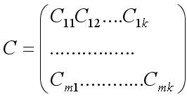
Where C 11 is the sum of the papar products of the elements of the row of matrix A and the column of matrix B, that is, the element is the sum of the product of the element of the first column of the first row of matrix A with the element of the first column of the first row of matrix B, the element of the second column of the first row of matrix A with the element of the first column of the second row matrices B, etc.
When multiplying, the order of the multiplication is important. A * B is not equal to B * A.
Finding the determinant.
Any square matrix can generate a determinant or determinant. Writes det. Or | matrix elements |
For matrices of dimension 2 by 2. Determine there is a difference between the product of elements of the main and elements of the side diagonal. 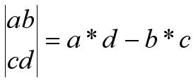
For matrices with dimensions 3 by 3 or more. The operation of finding the determinant is more complicated.
Let's introduce the concepts:
Element minor- is the determinant of the matrix obtained from the original matrix by deleting the row and column of the original matrix in which this element was located.
Algebraic complement element of a matrix is called the product of the minor of this element by -1 in the power of the sum of the row and column of the original matrix, in which this element was located.
The determinant of any square matrix is equal to the sum of the product of the elements of any row of the matrix by the corresponding algebraic complements.
Matrix inversion
Matrix inversion is the process of finding the inverse matrix that we defined at the beginning. The inverse matrix is also denoted as the original one with a postscript of the degree -1.
Find the inverse matrix by the formula.
A -1 = A * T x (1 / | A |)
Where A * T is the Transposed Matrix of Algebraic Complements.
We made examples of solving matrices in the form of a video tutorial
:
If you want to understand, look for sure.
These are the basic operations for solving matrices. If you have additional questions about how to solve matrices, feel free to write in the comments.
If, nevertheless, you could not figure it out, try to contact a specialist.
Matrix, familiarize yourself with its basic concepts. The defining elements of the matrix are its diagonals - and the side one. The main starts at the element in the first row, the first column, and continues to the element in the last column, the last row (that is, it goes from left to right). The side diagonal starts the other way around in the first row, but in the last column, and continues to the element that has the coordinates of the first column and the last row (goes from right to left).
In order to move on to the next definitions and algebraic operations on matrices, study the types of matrices. The simplest of them are square, unit, zero and inverse. The number of columns and rows is the same. The transposed matrix, let's call it B, is obtained from the matrix A by replacing columns with rows. In the one, all elements of the main diagonal are ones, and the others are zeros. And in zero, even the elements of the diagonals are zero. The inverse matrix is the one on which the original matrix comes to the unit form.
Also, the matrix can be symmetrical about the main or side axes. That is, the element with coordinates a (1; 2), where 1 is the row number and 2 is the column, is equal to a (2; 1). A (3; 1) = A (1; 3) and so on. Matrices consistent are those where the number of columns of one is equal to the number of rows of the other (such matrices can be multiplied).
The main actions that can be performed with matrices are addition, multiplication, and finding the determinant. If the matrices are of the same size, that is, they have the same number of rows and columns, then they can be added. It is necessary to add elements that are in the same places in the matrices, that is, add a (m; n) with in (m; n), where m and n are the corresponding coordinates of the column and row. When adding matrices, the main rule of ordinary arithmetic addition applies - when the places of the terms are changed, the sum does not change. Thus, if instead of a simple element a there is an expression a + b, then it can be added to an element from another commensurate matrix according to the rules a + (b + c) = (a + b) + c.
You can multiply the matched matrices given above. In this case, a matrix is obtained, where each element is the sum of the pairwise multiplied elements of the row of matrix A and the column of matrix B. When multiplying, the order of actions is very important. m * n is not equal to n * m.
Also one of the main actions is finding. It is also called a determinant and is denoted as det. This value is determined by the modulus, that is, it is never negative. The easiest way to find the determinant is for a 2x2 square matrix. To do this, multiply the elements of the main diagonal and subtract from them the multiplied elements of the secondary diagonal.