Axonometry is a parallel projection. Table 3.3 lists the first matrices of orthographic projections onto the coordinate planes obtained from their definitions.

Table 3.3 Design transformation and projection matrices

Orthographic projection on XOY		Orthographic projection on YOZ
Orthographic projection on XOZ		Orthographic projection onto the plane x = p
Trimetric transformation matrix on the XOY plane
Isometric transformation matrix to the XOY plane
XOY isometric projection matrix
Oblique projection matrix to XOY	Free projection matrix on XOY
XOY Cabinet Projection Matrix	Perspective transformation matrix with one vanishing point (picture plane perpendicular to the abscissa axis)
Perspective transformation matrix with one vanishing point (picture plane perpendicular to the ordinate)		Perspective transformation matrix with one vanishing point (picture plane perpendicular to the applicate axis)
Perspective transformation matrix with two vanishing points (picture plane parallel to the ordinate)		Perspective transformation matrix with three vanishing points (picture plane of arbitrary position)

Isometry, dimetry, and trimetry are obtained by combining rotations followed by a projection from infinity. If you need to describe the projection onto the XOY plane, then first you need to transform the rotation by an angle about the ordinate axis, then by the angle relative to the abscissa axis. Table 3.3 shows the trimetric transformation matrix. To obtain a matrix of dimetric transformation, in which, for example, the distortion coefficients along the abscissa and ordinate axes will be equal, the relationship between the angles of rotation must obey the dependence

That is, by choosing an angle , you can calculate the angle and determine the matrix of the dimetric projection. For an isometric transformation, the relationship of these angles turns into strictly defined values, which are:

Table 3.3 shows the isometric transformation matrix as well as the isometric projection matrix onto the XOY plane. The need for matrices of the first type lies in their use in algorithms for removing invisible elements.

In oblique projections, the projecting straight lines form an angle with the projection plane that differs from 90 degrees. Table 3.3 shows the general oblique projection matrix onto the XOY plane, as well as the free and cabinet projection matrices, in which:

Perspective projections (Table 3.3) are also represented by perspective transformations and perspective projections onto the XOY plane. V X, V Y and V Z are projection centers - points on the corresponding axes. –V X, –V Y, –V Z will be the points at which the bundles of straight lines parallel to the corresponding axes converge.

The observer's coordinate system is left coordinate system (Figure 3.3), in which the z e axis is directed from the point of view forward, the x e axis is directed to the right, and the y e axis is upward. Such a rule is adopted for the coincidence of the x e and y e axes with the x s and y s axes on the screen. Determining the values ​​of the screen coordinates x s and y s for point P leads to the need to divide by the coordinate z e. To build an accurate perspective view, it is necessary to divide by the depth coordinate of each point.

Table 3.4 shows the values ​​of the vertex descriptor S (X, Y, Z) of the model (Figure 2.1), subjected to rotational transformations and isometric transformations.

Table 3.4 Model Vertex Descriptors

Original model				M (R (z, 90)) xM (R (y, 90))

The engine does not move the ship.
The ship remains in place, and
engines move the universe
Around him.

Futurama

This is one of the most important lessons. Read it thoughtfully at least eight times.

Homogeneous coordinates

In the previous lessons, we assumed that the vertex is located at coordinates (x, y, z). Let's add one more coordinate - w. From now on, we will have the vertices at the coordinates (x, y, z, w)

You will soon understand what's what, but for now, take it for granted:

• If w == 1 then the vector (x, y, z, 1) is the position in space
• If w == 0 then the vector (x, y, z, 0) is the direction.

Remember this as an axiom without proof !!!

And what does it give us? Well, nothing for rotation. If you rotate a point or direction, you get the same result. But if you rotate the displacement (when you move the point in a certain direction), then everything changes dramatically. What does “shift direction” mean? Nothing special.

Homogeneous coordinates allow us to operate with a single device for both cases.

Transformation Matrices

Introduction to matrices

In simple terms, a matrix is ​​just an array of numbers with a fixed number of rows and columns.

For example, a 2-by-3 matrix would look like this:

In 3D graphics, we almost always use 4x4 matrices. This allows us to transform our (x, y, z, w) vertices. It's very simple - we multiply the position vector by the transformation matrix.

Matrix * Vertex = Transformed Vertex

It's not as scary as it looks. Point your left finger at a and your right finger at x. This will be ax. Move your left finger to the next number b and your right finger down to the next number y. We got by. Once again - cz. And again - dw. Now we sum up all the resulting numbers - ax + by + cz + dw. We got our new x. Repeat this for each line and you will get a new vector (x, y, z, w).

However, this is a rather boring operation, so let the computer do it for us.

In C ++ using the GLM library:

glm :: mat4 myMatrix;

glm :: vec4 myVector;

glm:: vec 4 transformedVector = myMatrix * myVector; // Don't forget about order !!! This is extremely important !!!

In GLSL:

mat4 myMatrix;

vec4 myVector;

// fill the matrix and vector with our values ​​... we skip this

vec 4 transformedVector = myMatrix * myVector; // just like in GLM

(Something seems to me that you did not copy this piece of code to your project and did not try it ... come on, try it, it's interesting!)

Displacement matrix

The displacement matrix is ​​probably the simplest matrix of all. There she is:

Here X, Y, Z are the values ​​we want to add to our vertex position.

So, if we need to move the vector (10,10,10,1) by 10 points, at position X, then:
(Try it yourself, well, please!)

... And we get (20,10,10,1) in a homogeneous vector. As I hope you remember, 1 means the vector is a position, not a direction.

Now let's try to transform the direction (0,0, -1,0) in the same way:

And in the end we got the same vector (0,0, -1,0).
As I said, it doesn't make sense to move the direction.

How do we code this?

In C ++ with GLM:

#include // after

glm :: mat4 myMatrix = glm :: translate (10.0f, 0.0f, 0.0f);

glm :: vec4 myVector (10.0f, 10.0f, 10.0f, 0.0f);

glm:: vec 4 transformedVector = myMatrix * myVector; // and what is the result?

And in GLSL: In GLSL, so rarely does anyone. Most often using the glm :: translate () function. First, they create a matrix in C ++, and then send it to GLSL, and already there they do only one multiplication:

vec4 transformedVector = myMatrix * myVector;

Identity Matrix

This is a special matrix. She doesn't do anything. But I mention it because it's important to know that multiplying A by 1.0 yields A:

glm :: mat4 myIdentityMatrix = glm :: mat4 (1.0f);

Scaling Matrix

The scaling matrix is ​​also pretty simple:

So if you want to double the vector (position or direction, it doesn't matter) in all directions:

And the w coordinate has not changed. If you ask, "What is direction scaling?" Not often useful, but sometimes useful.

(note that scaling the identity matrix with (x, y, z) = (1,1,1))

C ++:

// Use#include and#include

glm :: mat4 myScalingMatrix = glm :: scale (2.0f, 2.0f, 2.0f);

Rotation Matrix

But this matrix is ​​quite complicated. Therefore, I will not dwell on the details of its internal implementation. If you really want to, you better read (Matrices and Quaternions FAQ)

VWITH++:

// Use#include and#include

glm :: vec3 myRotationAxis (??, ??, ??);

glm :: rotate (angle_in_degrees, myRotationAxis);

Composite Transforms

We now know how to rotate, move and scale our vectors. It would be nice to know how to combine all this. This is done simply by multiplying the matrices with each other.

TransformedVector = TranslationMatrix * RotationMatrix * ScaleMatrix * OriginalVector;

And again the order !!! First you need to resize, then scroll and only then move.

If we apply transformations in a different order, we will not get the same result. Try it:

• Take a step forward (don't knock the computer off the table) and turn left
• Turn left and take one step forward.

Yes, you must always remember about the order of actions when controlling, for example, a game character. First, if necessary, do the scaling, then set the direction (rotation) and then move. Let's take a look at a small example (I removed rotation to make calculations easier):

Wrong way:

• Move the ship to (10,0,0). Its center is now 10 X from the center.
• We increase the size of our ship 2 times. Each coordinate is multiplied by 2 relative to the center, which is far away ... And as a result, we get a ship of the required size, but in position 2 * 10 = 20. Which is not exactly what we wanted.

The right way:

• We increase the size of the ship by 2 times. We now have a large ship in the center.
• We move the ship. The size of the ship has not changed and it is located in the right place.

Matrix-matrix multiplication is done in much the same way as matrix-vector multiplication. We will not go into details, but let the curious read it from specialized sources. We're just going to rely on the GLM library.
ВС ++:
glm :: mat4 myModelMatrix = myTranslationMatrix * myRotationMatrix * myScaleMatrix;
glm :: vec4 myTransformedVector = myModelMatrix * myOriginalVector;
In GLSL:
mat4 transform = mat2 * mat1;
vec4 out_vec = transform * in_vec;

Model, View and Projection Matrices

For illustration purposes, we will assume that we already know how to draw in OpenGL our favorite 3D model of Blender - the head of Suzanne the monkey.

The Model, View and Projection matrices are a very convenient method for separating transformations. You don't have to use them if you really want to (we didn't use them in Lessons 1 and 2). But I strongly recommend that you use them. It's just that almost all 3D libraries, games, etc. use them to separate transformations.

Model Matrix

This model, like our beloved triangle, is defined by a set of vertices. X, Y, Z coordinates are specified relative to the center of the object. So, if the vertex is located at coordinates (0,0,0), then it is in the center of the entire object

We are now able to move our model. For example, because the user controls it with the keyboard and mouse. It's very easy to do: scaling * rotating * moving and that's it. You apply your matrix to all vertices in every frame (in GLSL, not C ++) and everything moves. Everything that does not move is located in the center of the "world".

The vertices are in world space The black arrow in the figure shows how we go from model space to world space (All vertices were specified relative to the center of the model, and steel were specified relative to the center of the world)

This transformation can be displayed with the following diagram:

View Matrix

Let's read the quote from futurama again:

“The engine does not move the ship. The ship remains in place, and the engines move the universe around it. "

The same can be applied to the camera. If you want to photograph a mountain from any angle, you can move the camera ... or the mountain. This is impossible in real life, but it is very easy and convenient in computer graphics.

By default, our camera is in the center of the World Coordinates. To move our world, we need to create a new matrix. For example, we need to move our camera 3 units to the right (+ X). This is the same as moving the whole world 3 units to the left (-X). And while your brains are melting, let's try:

// Use #include and #include

glm :: mat4 ViewMatrix = glm :: translate (-3.0f, 0.0f, 0.0f);

The picture below demonstrates this: we are moving from World space (all vertices are set relative to the center of the world as we did in the previous section) to camera space (all vertices are set relative to the camera).

And before your head explodes completely, check out this great function from our good old GLM:

glm :: mat4 CameraMatrix = glm :: LookAt (

cameraPosition, // Camera Position In World Coordinates

cameraTarget, // the point we want to look at in world coordinates

upVector// most likely glm:: vec3 (0,1,0), and (0, -1,0) will show everything upside down, which is sometimes cool too.

Here's an illustration to the above:

But to our delight, that's not all.

Projection Matrix

Now we have coordinates in camera space. This means that after all these transformations, the vertex of which is lucky enough to be at x == 0 and y == 0 will be rendered in the center of the screen. But we can't just use the X, Y coordinates to figure out where to draw the vertex: the distance to the camera (Z) must also be taken into account! If we have two vertices, then one of them will be closer to the center of the screen than the other, since it has a larger Z coordinate.

This is called perspective projection:

And fortunately for us, a 4x4 matrix can also represent perspective transformations:

glm :: mat4 projectionMatrix = glm :: perspective (

FoV, // Horizontal Field of View in degrees. Or magnitudeapproximations. Howas if « lens» on thecamera. Usually between 90 (super wide, like a fisheye) and 30 (like a small spyglass)

4.0 f / 3.0 f, // Aspect ratio. Depends on the size of your window. For example, 4/3 == 800/600 == 1280/960 sounds familiar, doesn't it?

0.1 f, // Near clipping field. It should be set as large as possible, otherwise there will be problems with accuracy.

100.0 f // Far clipping field. It should be kept as small as possible.

);

Let's repeat what we have done now:

We have moved away from camera space (all vertices are set in coordinates relative to the camera) into homogeneous space (all vertices are in coordinates of a small cube (-1,1). Everything in the cube is on the screen.)

And the final diagram:

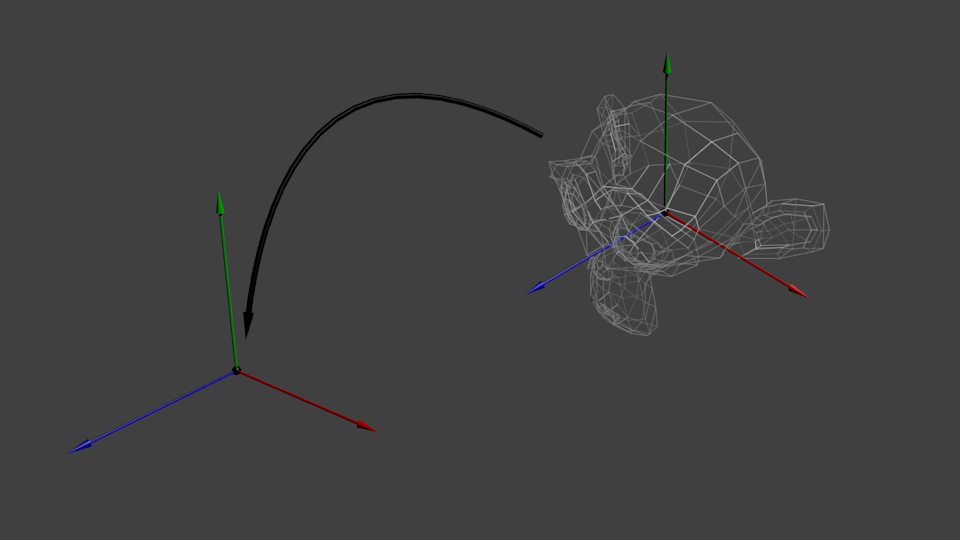
Here's another picture to make it clearer what happens when we multiply all this projection matrix nonsense. Before multiplying by the projection matrix, we have blue objects defined in camera space and a red object that represents the camera's view field: the space that falls into the camera lens:

After multiplying by the projection matrix, we get the following:

In the previous picture, the view field has turned into a perfect cube (with vertex coordinates from -1 to 1 in all axes.), And all objects are deformed in perspective. All blue objects that are close to the camera have become large, and those farther - small. The same as in life!

Here is the view we have from the "lens":

However, it is square, and one more mathematical transformation needs to be applied to fit the picture to the size of the window.

In order to rotate objects (or a camera), a serious mathematical basis is needed, with the help of which the coordinates of all objects will be calculated when displayed on a "flat" computer screen. I want to say right away that you should not be intimidated, all mathematical libraries have already been written for us, we will only use them. In any case, the following text does not need to be skipped, regardless of the level of knowledge of mathematics.

1. Matrices, general concepts

What are matrices? We recall higher mathematics: a matrix ¬ is a set of numbers with a previously known dimension of rows and columns.

Matrices can be added, multiplied by a number, multiplied with each other and many other interesting things, but we will skip this moment, because it is described in sufficient detail in any textbook on higher mathematics (textbooks can be searched on google.com). We will use matrices as programmers, we fill them in and say what to do with them, all calculations will be performed by the Direct3D mathematical library, so you need to include the d3dx9.h header module (and the d3dx9.lib library) in the project.

Our task is to create an object, i.e. fill the matrix with the coordinates of the object's vertices. Each vertex is a vector (X, Y, Z) in 3D space. Now, in order to perform some action, we need to take our object (that is, the matrix) and multiply by the transformation matrix, the result of this operation is a new object specified in the form of a matrix.

There are three main matrices defined and used in Direct3D: world matrix, view matrix, and projection matrix. Let's consider them in more detail.

World Matrix- allows for rotation, transformation and scaling of an object, and also endows each of the objects with its own local coordinate system.

Functions for working with the world matrix:

D3DXMatrixRotationX (), D3DXMatrixRotationY (), D3DXMatrixRotationZ () - point rotation about one of the axes;

D3DXMatrixTranslation () - move a point to another position;

D3DXMatrixScale () - scaling.

View Matrix- defines the location of the scene viewing camera and can consist of any combination of broadcast and rotation.
D3DXMatrixLookAtLH () and D3DXMatrixLookAtRH () define the camera position and viewing angle for the left-handed and right-handed coordinate systems, respectively.

Projection Matrix- creates a projection of a 3D scene onto the monitor screen. It transforms the object, moves the origin to the front, and defines the front and back clipping planes.

By filling in these matrices and making transformations, you create a three-dimensional scene in which you get the ability to move, rotate, zoom in, remove and perform other actions on objects, depending on your needs.

2. Object creation

We create a new project, similar to the first one. Before we continue to complicate our code, let's break it down into parts for better readability of the code. It is logical to divide our project into three components:

1. Windows window (window initialization, messages, ...)
2. 3D initialization (loading object coordinates, deleting resources, ...)
3. Scene rendering (matrices, drawing primitives, ...)

As a result, we will have 3 files - window.cpp, init3d.h, render.h with the following content: init3d.h- we transfer global variables and structures, declaration of functions, functions InitDirectX (), InitBufferVertex (), Destroy3D () render.h- we transfer the RenderScene () function, everything that remains touches the main window, it will be a file - window.cpp.

Adding a header file and library for using matrix functions

#include // or C: \ DXSDK \ Include \ d3dx9.h #pragma comment (lib, "d3dx9.lib") // or C: \\ DXSDK \\ Lib \\ d3dx9.lib

We also need standard functions for working with time, so we include the appropriate header file:

#include

Let's change the format of vertex representation:

#define D3DFVF_CUSTOMVERTEX (D3DFVF_XYZ / D3DFVF_DIFFUSE) struct CUSTOMVERTEX ( Float x, y, z; DWORD color; );

We will use an unconverted vertex type, since transformations will be done by matrices.
Change the code of the InitDirectX () function. The setting of two display modes must be added to this function.
Turn off the clipping mode so that when you rotate you can see all sides of the object:

PDirectDevice-> SetRenderState (D3DRS_CULLMODE, D3DCULL_NONE);

At the moment, we are not using lighting, but painting the vertices in a certain color, so we turn off the lighting:

PDirectDevice-> SetRenderState (D3DRS_LIGHTING, FALSE);

Let's simplify our heart by presenting it as three triangles. We will use a local coordinate system.

CUSTOMVERTEX stVertex = ((-1.0f, 0.5f, 0.0f, 0x00ff0000), (-0.5f, 1.0f, 0.0f, 0x00ff0000), (0.0f, 0.5f, 0.0f, 0x00ff0000), (0.0f, 0.5 f, 0.0f, 0x000000ff), (0.5f, 1.0f, 0.0f, 0x000000ff), (1.0f, 0.5f, 0.0f, 0x000000ff), (-1.0f, 0.5f, 0.0f, 0x0000ff00), (1.0 f, 0.5f, 0.0f, 0x0000ff00), (0.0f, -1.0f, 0.0f, 0x0000ff00),);

3. Creation of transformation matrices

Let's write in the render.h file the SetupMatrix () function in which all actions on matrices will take place.

Let's create matrices:

D3DXMATRIX MatrixWorld; - world matrix

D3DXMATRIX MatrixView; - matrix of the form

D3DXMATRIX MatrixProjection; - projection matrix
Setting the world matrix

In order for the object to rotate, it is necessary to get the system time and every "instant" change the angle between the local coordinate system and the world coordinate system. We will rotate about the X axis, so we use the D3DXMatrixRotationX function. After calculating the world matrix, you need to apply its values ​​using the SetTransform function:

UINT iTime = timeGetTime ()% 5000; FLOAT fAngle = iTime * (2.0f * D3DX_PI) /5000.0f; D3DXMatrixRotationX (& MatrixWorld, fAngle); pDirectDevice-> SetTransform (D3DTS_WORLD, & MatrixWorld); Setting the view matrix

Install the camera in the right place and direct it to the object

D3DXMatrixLookAtLH (& MatrixView, - the result of the function

& D3DXVECTOR3 (0.0f, 0.0f, -8.0f), - the point at which the camera is located

& D3DXVECTOR3 (0.0f, 0.0f, 0.0f), - the point at which we are looking

& D3DXVECTOR3 (0.0f, 1.0f, 0.0f)); - the top of the object

After calculation, you need to apply the obtained values.

The engine does not move the ship. The ship remains in place, and the engine moves the universe relative to it.

This is a very important part of the lessons, be sure to read it several times and understand it well.

Homogeneous coordinates

Until now, we have operated with 3-dimensional vertices as (x, y, z) triplets. Let us introduce one more parameter w and operate with vectors of the form (x, y, z, w).

Remember forever that:

• If w == 1, then the vector (x, y, z, 1) is a position in space.
• If w == 0, then the vector (x, y, z, 0) is the direction.

What does it give us? Ok, this does not change anything for rotation, since in the case of a point rotation and in the case of a direction vector rotation, you get the same result. However, in the case of transfer, there is a difference. Moving the direction vector will give the same vector. We will dwell on this in more detail later.

Homogeneous coordinates allow us to operate with vectors in both cases using one mathematical formula.

Transformation matrices

Introduction to matrices

The easiest way to imagine a matrix is ​​as an array of numbers, with a strictly defined number of rows and columns. For example, a 2x3 matrix looks like this:

However, in 3D graphics we will only use 4x4 matrices which will allow us to transform our vertices (x, y, z, w). The transformed vertex is the result of multiplying the matrix by the vertex itself:

Matrix x Vertex (in that order !!) = Transform. vertex

Pretty simple. We'll be using this quite often, so it makes sense to instruct a computer to do this:

In C ++ using GLM:

glm :: mat4 myMatrix; glm :: vec4 myVector; glm :: // Pay attention to the order! He's important!

In GLSL:

mat4 myMatrix; vec4 myVector; // Don't forget to fill the matrix and vector with the required values ​​here vec4 transformedVector = myMatrix * myVector; // Yes, this is very similar to GLM :)

Try experimenting with these snippets.

Transfer matrix

The transfer matrix looks like this:

where X, Y, Z are the values ​​we want to add to our vector.

So, if we want to move the vector (10, 10, 10, 1) by 10 units in the X direction, then we get:

… We get (20, 10, 10, 1) homogeneous vector! Do not forget that 1 in the w parameter means position, not direction, and our transformation did not change the fact that we are working with position.

Now let's see what happens if the vector (0, 0, -1, 0) is a direction:

... and we get our original vector (0, 0, -1, 0). As it was said before, the vector with the parameter w = 0 cannot be transferred.

And now is the time to move that into the code.

In C ++, with GLM:

#include // after glm :: mat4 myMatrix = glm :: translate (glm :: mat4 (), glm :: vec3 (10.0 f, 0.0 f, 0.0 f)); glm :: vec4 myVector (10.0 f, 10.0 f, 10.0 f, 0.0 f); glm :: vec4 transformedVector = myMatrix * myVector;

In GLSL:

vec4 transformedVector = myMatrix * myVector;

In fact, you will never do this in the shader, most often you will execute glm :: translate () in C ++ to compute the matrix, pass it to GLSL, and then perform the multiplication in the shader.

Unit Matrix

This is a special matrix that doesn't do anything, but we're touching it, as it's important to remember that A multiplied by 1.0 gives A:

In C ++:

glm :: mat4 myIdentityMatrix = glm :: mat4 (1.0 f);

Scaling matrix

Looks simple as well:

So, if you want to apply vector scaling (position or direction - it doesn't matter) by 2.0 in all directions, then you need to:

Note that w does not change, and also note that the identity matrix is ​​a special case of a scaling matrix with a scale factor of 1 on all axes. Also, the identity matrix is ​​a special case of the transfer matrix, where (X, Y, Z) = (0, 0, 0), respectively.

In C ++:

// add #include and #include glm :: mat4 myScalingMatrix = glm :: scale (2.0 f, 2.0 f, 2.0 f);

Rotation matrix

More difficult than previously discussed. We'll skip the details here as you don't need to know for sure for daily use. For more information, you can follow the link Matrices and Quaternions FAQ (quite a popular resource and perhaps your language is available there)

In C ++:

// add #include and #include glm :: vec3 myRotationAxis (??, ??, ??); glm :: rotate (angle_in_degrees, myRotationAxis);

Putting transformations together

So now we can rotate, translate and scale our vectors. The next step would be nice to combine transformations, which is implemented using the following formula:

TransformedVector = TranslationMatrix * RotationMatrix * ScaleMatrix * OriginalVector;

ATTENTION! This formula actually shows that the scaling is done first, then the rotation, and only last is the translation. This is how matrix multiplication works.

Be sure to remember in what order all this is done, because the order is really important, in the end you can check it yourself:

• Take a step forward and turn left
• Turn left and take a step forward

The difference is really important to understand, as you will constantly be faced with this. For example, when you work with game characters or some objects, always zoom first, then rotate, and only then transfer.

In fact, the above order is what you usually need for playable characters and other items: first scale it up if needed; then set its direction and then move it. For example, for a ship model (turns removed for simplicity):

• Wrong Way:
  • You move the ship to (10, 0, 0). Its center is now 10 units from the origin.
  • You scale your ship 2x. Each coordinate is multiplied by 2 "relative to the original", which is far ... So, you find yourself in a large ship, but its center is 2 * 10 = 20. Not what you wanted.
• The right way:
  • You scale your ship 2x. You get a large ship centered at the origin.
  • You are carrying your ship. It is still the same size and at the correct distance.

In C ++, with GLM:

glm :: mat4 myModelMatrix = myTranslationMatrix * myRotationMatrix * myScaleMatrix; glm :: vec4 myTransformedVector = myModelMatrix * myOriginalVector;

In GLSL:

mat4 transform = mat2 * mat1; vec4 out_vec = transform * in_vec;

World, view and projection matrices

For the rest of this tutorial, we will assume that we know how to display our favorite 3D model from Blender - Suzanne the monkey.

World, view and projection matrices are a convenient tool for separating transformations.

World Matrix

This model, just like our red triangle, is set by a set of vertices, the coordinates of which are set relative to the center of the object, that is, the vertex with coordinates (0, 0, 0) will be in the center of the object.

Next, we would like to move our model, since the player controls it using the keyboard and mouse. All we do is scale, then rotate and translate. These actions are performed for each vertex, in each frame (performed in GLSL, not in C ++!) And thus our model moves on the screen.

Now our peaks are in world space. This is shown by the black arrow in the figure. We have moved from object space (all vertices are relative to the center of the object) to world space (all vertices are relative to the center of the world).

It is shown schematically as follows:

View matrix

To quote Futurama again:

The engine does not move the ship. The ship remains in the same place, and the engine moves the universe around it.

Try to imagine this in relation to the camera. For example, if you want to photograph a mountain, then you do not move the camera, but move the mountain. This is not possible in real life, but it is incredibly simple in computer graphics.

So, initially, your camera is at the center of the world coordinate system. To move the world you need to enter another matrix. Let's say you want to move the camera 3 units RIGHT (+ X), which is the equivalent of moving the entire world 3 units LEFT (-X). In the code, it looks like this:

// Add #include and #include glm :: mat4 ViewMatrix = glm :: translate (glm :: mat4 (), glm :: vec3 (- 3.0 f, 0.0 f, 0.0 f));

Again, the image below fully illustrates this. We switched from the world coordinate system (all vertices are specified relative to the center of the world system) to the camera coordinate system (all vertices are specified relative to the camera):

And while your brain is digesting this, we will take a look at the function that GLM provides us, or rather glm :: LookAt:

glm :: mat4 CameraMatrix = glm :: LookAt (cameraPosition, // The position of the camera in world space cameraTarget, // Indicates where you are looking in world space upVector // A vector pointing upwards. Usually (0, 1, 0));

And here is a diagram that shows what we are doing:

However, this is not the end.

Projection matrix

So now we are in camera space. This means that the vertex that receives the coordinates x == 0 and y == 0 will be displayed in the center of the screen. However, when displaying an object, the distance to the camera (z) also plays a huge role. For two vertices with the same x and y, the vertex with the higher z value will appear closer than the other.

This is called perspective projection:

And luckily for us, a 4x4 matrix can do this projection:

// Creates a really hard-to-read matrix, but nonetheless this is a standard 4x4 matrix glm :: mat4 projectionMatrix = glm :: perspective (glm :: radians (FoV), // Vertical field of view in radians. Typically between 90 ° (very wide) and 30 ° (narrow) 4.0 f / 3.0 f, // Aspect ratio. Depends on the size of your window. Note that 4/3 == 800/600 == 1280/960 0.1 f, // Near clipping plane. Must be greater than 0. 100.0 f // Far clipping plane.);

We moved from Camera Space (all vertices are set relative to the camera) to Homogeneous space (all vertices are in a small cube. Everything inside the cube is displayed).

Now let's take a look at the following images so that you can better understand what is happening with the projection. Before projection, we have blue objects in camera space, while the red shape shows the view of the camera, that is, everything that the camera sees.

The use of the Projection Matrix has the following effect:

In this image, the camera view is a cube and all objects are deformed. Objects closer to the camera appear large, and those farther away appear small. Just like in reality!

This is how it will look:

The image is square, so the following mathematical transformations are applied to stretch the image to fit the actual window size:

And this image is what will actually be displayed.

Merging transformations: the ModelViewProjection matrix

... Just the standard matrix transformations you already love!

// C ++: calculating the matrix glm :: mat4 MVPmatrix = projection * view * model; // Remember! In reverse order!

// GLSL: Apply The Matrix transformed_vertex = MVP * in_vertex;

Putting it all together

• The first step is to create our MVP matrix. This must be done for every model you display.

// Projection Array: 45 ° Field of View, 4: 3 Aspect Ratio, Range: 0.1 unit<->100 units glm :: mat4 Projection = glm :: perspective (glm :: radians (45.0 f), 4.0 f / 3.0 f, 0.1 f, 100.0 f); // Or, for orthocamera glm :: mat4 View = glm :: lookAt (glm :: vec3 (4, 3, 3), // The camera is in world coordinates (4,3,3) glm :: vec3 (0, 0, 0), // And directed to the origin glm :: vec3 (0, 1, 0) // "Head" is on top); // Model matrix: identity matrix (Model is at the origin) glm :: mat4 Model = glm :: mat4 (1.0 f); // Individually for each model // The resulting ModelViewProjection matrix, which is the result of multiplying our three matrices glm :: mat4 MVP = Projection * View * Model; // Remember that matrix multiplication is done in reverse order

• The second step is to pass this to GLSL:

// Get the handle to the variable in the shader // Only once during initialization. GLuint MatrixID = glGetUniformLocation (programID, "MVP"); // Pass our transformations to the current shader // This is done in the main loop, since each model will have a different MVP matrix (at least part of M) glUniformMatrix4fv (MatrixID, 1, GL_FALSE, & MVP [0] [0]);

• The third step is to use the received data in GLSL to transform our vertices.

// Vertex input data, different for all executions of this shader. layout (location = 0) in vec3 vertexPosition_modelspace; // Values ​​that remain constant for the entire grid. uniform mat4 MVP; void main () ( // Output position of our vertex: MVP * position gl_Position = MVP * vec4 (vertexPosition_modelspace, 1); )

• Ready! Now we have the same triangle as in Lesson 2, still located at the origin (0, 0, 0), but now we see it in perspective from point (4, 3, 3).

In Lesson 6, you will learn how to dynamically change these values ​​using your keyboard and mouse to create the camera that you are used to seeing in games. But first we will learn how to give our models colors (Lesson 4) and textures (Lesson 5).

Tasks

• Try changing the glm :: perspective values
• Instead of using perspective projection, try using orthographic (glm: ortho)
• Modify ModelMatrix to move, rotate and scale the triangle
• Use the previous task, but with a different order of operations. Pay attention to the result.

Perspective projection

We have considered important projections used in affine geometry. Now let's move on to considering perspective geometry and several new types of projection.

In photographs, paintings, the screen, the images seem natural and correct to us. These images are called perspective images. Their properties are such that more distant objects are depicted on a smaller scale, parallel lines are generally not parallel. As a result, the geometry of the image turns out to be quite complex, and it is difficult to determine the size of certain parts of the object from the finished image.

A conventional perspective projection is a central projection onto a plane with straight rays passing through a point - the center of the projection. One of the projection rays is perpendicular to the projection plane and is called the main one. The point of intersection of this ray and the projection plane is the main point of the picture.

There are three coordinate systems. Usually a programmer works and keeps data about geometric objects in world coordinates. To increase the realism in preparation for displaying the image on the screen, data about objects from world coordinates is converted into view coordinates. And only at the moment of displaying the image directly on the display screen do they move to screen coordinates, which are the numbers of screen pixels.

The first two systems can be used in multidimensional coordinate systems, but the latter only in 2D. Operations are irreversible, that is, it is impossible to restore a three-dimensional image from a two-dimensional projection image.

In this matrix, the elements a, d, e are responsible for scaling, m, n, L- for displacement, p, q, r- for projecting, s- for complex scaling, X- for rotation.

One-point projection onto the z = 0 plane

The essence of this projection is as follows: the deeper the object is, the larger the value of the z-coordinate and the denominator rz + 1 becomes, and, therefore, the smaller the object looks on the projection plane. Let's perform simple calculations and explain them graphically:
the equation x "/ F = x / (F + z pr) is equivalent to: x" = xF / (F + z pr) = x / (1 + z pr / F) = x / (1 + rz pr), where r = 1 / F, F - focus.

For points lying on a line parallel to the axis z, did not get lost one after another, one-point projection onto the line is used (see transformation matrix and rice. 4.2); the z-coordinate has disappeared, but since distant objects have become smaller than similarly close ones, the viewer has a sense of depth. Remember: this is the first way to convey depth on a plane!