If you do not know how to create a table in Excel, then go through Start, All Programs, Microsoft Office, Excel , no matter what version. In the menu, click create a new document, or press the key combination ctrl + N. Immediately save the file under a meaningful name and in an accessible place.
Depending on what kind of excel table we need and what we need, we will do this: the first row will be the table header. Let's add column names to each cell horizontally.
Creating an excel spreadsheet, the basics

The address range will be such and such A1:Z1, for example. We enter the data of the table by columns into the range A2: Z100, for example. You will most likely have fewer rows and columns.
 If you have a column with a date, and in the cell after typing 11/11/2011 something similar to 41853 is obtained, then you need to right-click on the cell and select Format Cell in the context menu. Or press ctrl+1. In the second tab, select the date type.
 Actually, this will most likely need to be done with the entire column ... If you need to enter a number starting from zero, for example 007, then either select the text format in the cell format, or write a single quote "007 like this. Very reliable. Otherwise, you the cell will just contain the number 7.
 When the data is entered, do not forget to save the file, but it is better to do this from time to time. Of course, you can set auto-save in the settings after a short period of time, but at the same time you lose the ability to undo the last actions. If something is not typed or not there.
 Let's start designing the table: on the excel ribbon, select the icon with the grid, see which one suits best, select all the useful data along with the header and click on the icon with the grid. The table is almost ready, you can select the header, make the font bold and fill the cells with light gray. If an excel table needs to be printed, then such a gray header makes it very easy to read the data. Change the font size, go to the Preview menu. If the entire table fits on a sheet, consider yourself lucky.
 If not, then go to View Page Layout Page View. A blue frame will appear around the grid, move its borders so that the entire table fits. You may need to change the page view from portrait to landscape. Save the file and then either print it or mail it. What is a good way to have the table header in the first row, and not in the third or fifth? It seems that you can also place it in the center of the screen and indicate the margins of the fields in the markup.
 But, firstly, it is easier to filter the table from the first row than if you have a table block elsewhere. In addition, it is very convenient to export a table in this form to access as a database, or to sqlite3 if you will use
Microsoft Excel is a very powerful tool, thanks to which you can create large spreadsheets with a beautiful design and an abundance of various formulas. Working with information is facilitated precisely because of the dynamics that are missing in the Word application.
This article will show you how to create a table in Excel. Thanks to step-by-step instructions, even a "teapot" can figure it out. At first, novice users may find this difficult. But in fact, with constant work in the Excel program, you will become a professional and be able to help others.
The training plan will be simple:
- first, consider the various methods for creating tables;
- Then we are engaged in design so that the information is as clear and understandable as possible.
This method is the simplest. This is done in the following way.
- When you open a blank sheet, you will see a large number of identical cells.

- Select any number of rows and columns.

- After that, go to the "Home" tab. Click on the "Borders" icon. Then select "All".

- Immediately after that, you will have the usual elementary tablet.

Now you can start filling in the data.
There is another way to manually draw a table.
- Click on the "Borders" icon again. But this time, select Draw Grid.

- Immediately after that, you will change the appearance of the cursor.

- Make a left mouse click and drag the pointer to another position. As a result, a new grid will be drawn. The upper left corner is the initial position of the cursor. The lower right corner is the end.

The sizes can be any. The table will be created until you release your finger from the mouse button.
Auto mode
If you do not want to "work with your hands", you can always use ready-made functions. To do this, do the following.
- Go to the "Insert" tab. Click on the "Tables" button and select the last item.

Pay attention to what we are prompted about hot keys. In the future, for automatic creation, you can use the combination of buttons Ctrl + T .
- Immediately after that, you will see a window in which you need to specify the range of the future table.

- To do this, simply select any area - the coordinates will be substituted automatically.

- As soon as you release the cursor, the window will return to its original form. Click on the "OK" button.

- As a result of this, a beautiful table with alternating lines will be created.

- To change the name of a column, just click on it. After that, you can start editing directly in this cell or in the formula bar.

pivot table
This type of information presentation serves for its generalization and subsequent analysis. To create such an element, you need to do the following steps.
- First, we create a table and fill it with some data. How to do this is described above.

- Now go to the main menu "Insert". Next, we choose the option we need.

- Right after that, you will have a new window.

- Click on the first line (the input field must be made active). Only after that we select all the cells.

- Then click on the "OK" button.

- As a result of this, you will have a new sidebar where you need to configure the future table.

- At this stage, you need to transfer the fields to the desired categories. The columns will be months, the rows will be the purpose of the costs, and the values will be the amount of money.

To transfer, left-click on any field and, without releasing your finger, drag the cursor to the desired location.

Only after that (the cursor icon will change appearance) can the finger be released.

- As a result of these actions, you will have a new beautiful table in which everything will be calculated automatically. Most importantly, new cells will appear - “Grand Total”.

You can specify the fields that are of interest for data analysis.
Sometimes it is not possible to correctly select fields for columns and rows. And in the end, nothing worthwhile comes out. For such cases, Microsoft developers have prepared their own data analysis options.
It works very simply.
- First of all, we select the information we need.

- After that, select the appropriate menu item.

- As a result, the program itself will analyze the contents of the cells and offer several options.

- By clicking on any of the proposed options and clicking on the "OK" button, everything will be created automatically.

- In the case of the example, we got the sum of the total costs, excluding months.

Ready-made templates in Excel 2016
For those who are especially lazy, this program allows you to create truly “cool” tables with just one click.
When you open Excel, you have the following options to choose from:
- open the latest files you have worked with before;
- create a new empty workbook;
- see a tutorial with detailed information about the capabilities of this software;
- choose some ready-made default template;
- continue searching on the Internet if you don’t like any of the proposed designs;
- sign in with your Microsoft account.

We are interested in ready-made options. If you scroll down a bit, you will see that there are a lot of them. But these are the default templates. Imagine how many you can download them on the Internet.

Click on any option you like.
Click on the "Create" button.

As a result of this, you get a ready-made version of a very large and complex table.

Decor
Appearance is one of the most important parameters. It is very important to focus on some elements. For example, a header, title, and so on. Everything depends on the specific case.
Consider briefly the basic manipulations with cells.
Create a header
Let's use a simple table as an example.

- First, go to the "Home" tab and click on the menu item "Insert Rows to Sheet".

- Select the line that appears and click on the "Merge Cells" menu item.

- Next, write any title.

Changing the Height of Elements
Our header is the same size as the header. And it's not very pretty. In addition, it looks inconspicuous. In order to fix this, you need to move the cursor to the border of lines 1 and 2. After its appearance changes, left-click and drag it down.

As a result, the row height will be larger.

Text alignment
Our title is at the bottom of the cell and stuck to the header. In order to fix this, you need to use the alignment buttons. You can change the text position both vertically and horizontally.

We click on the button "In the middle" and we get the desired result.

Now the title looks much better.

Style change

Or use predefined styles. To do this, first select the line. Then, through the menu, select any of the proposed design options.

The effect will be very beautiful.

How to insert a new row or column
In order to change the number of elements in the table, you can use the "Insert" button.

You can add:
- cells;
- lines;
- columns;
- whole sheet.
Removing elements
You can destroy a cell or something else in the same way. There is a button for this.

Filling cells
If you want to highlight any column or line, you need to use the fill tool for this.

Thanks to it, you can change the color of any cells that were previously selected.

Element Format
You can do whatever you want with the table. To do this, just click on the "Format" button.

As a result of this, you will be able to:
- manually or automatically change the height of the rows;
- manually or automatically change the width of the columns;
- hide or show cells;
- rename sheet;
- change label color;
- protect the sheet;
- block the element;
- specify the cell format.
Content Format
If you click on the last of the above items, the following will appear:

With this tool, you can:
- change the format of the displayed data;
- specify alignment;

- choose any font;

- change table borders;

- "play" with the fill;

- set protection.

Using formulas in tables
It is thanks to the ability to use the auto-calculation functions (multiplication, addition, and so on) that Microsoft Excel has become a powerful tool.

In addition, it is recommended to read the description of all functions.

Consider the simplest operation - cell multiplication.
- First, let's prepare the field for experiments.

- Make active the first cell in which you want to display the result.

- Enter the following command there.

- Now press the Enter key. After that, move the cursor over the lower right corner of this cell until its appearance changes. Then hold down the left mouse click with your finger and drag down to the last line.

- As a result of autosubstitution, the formula will fall into all cells.

The values in the "Total cost" column will depend on the "Quantity" and "Cost per 1 kg" fields. That's the beauty of dynamics.
In addition, you can use ready-made functions for calculations. Let's try to calculate the sum of the last column.
- First, select the values. Then click on the "Autosums" button, which is located on the "Home" tab.

- As a result of this, the total sum of all numbers will appear below.

Use of graphics
Sometimes photos are used in cells instead of text. It is very easy to do this.
Select an empty element. Go to the "Insert" tab. Select the "Illustrations" section. Click on "Pictures".

- Specify the file and click on the "Insert" button.

- The result will not disappoint you. Looks very nice (depending on the selected pattern).

Export to Word
In order to copy data into a Word document, it is enough to do a couple of simple steps.
- Select the data area.

- Press the hotkeys Ctrl +C .
- Open Document
- Now use the buttons Ctrl + V .
- The result will be as follows.

Online Services
For those who want to work in "real mode" and share information with friends or work colleagues, there is a great tool.

Using this service, you can access your documents from any device: computer, laptop, phone or tablet.
Printing methods
Printing Word documents is usually a simple task. But with tables in Excel, everything is different. The biggest problem is that "by eye" it is difficult to determine the boundaries of the print. And very often almost empty sheets appear in the printer, on which there are only 1-2 lines of the table.
Such printouts are inconvenient for perception. It is much better when all the information is on one sheet and does not go anywhere beyond the borders. In this regard, developers from Microsoft have added the function of viewing documents. Let's see how to use it.
- We open the document. He looks quite normal.

- Next, press the hot keys Ctrl + P . In the window that appears, we see that the information does not fit on one sheet. We have lost the column "Total cost". In addition, at the bottom we are prompted that 2 pages will be used for printing.

In the 2007 version, for this you had to click on the "View" button.
- To cancel, press the hot key Esc. As a result, a vertical dotted line will appear, which shows the borders of the print.

You can increase the space when printing as follows.
- First of all, we reduce the margins. To do this, go to the "Page Layout" tab. Click on the "Fields" button and select the most "Narrow" option.

- After that, reduce the width of the columns until the dotted line is outside the last column. How to do this was described above.

You need to reduce it within reasonable limits so that the readability of the text does not suffer.
- Press Ctrl+P again. Now we see that the information is placed on one sheet.

Microsoft Product Version Differences
It should be understood that Excel 2003 has long been obsolete. It lacks a huge number of modern features and capabilities. In addition, the appearance of various objects (graphs, diagrams, and so on) is much inferior to modern requirements.
An example of an Excel 2003 workspace.

In modern 2007, 2010, 2013, and even more so 2016 versions, everything is much “cooler”.

Many menu items are in different sections. Some of them even changed their name. For example, the “Formulas” familiar to us were called “Functions” back in 2003. And they didn't take up much space.

Now they have a whole tab dedicated to them.

Limitations and features of different versions
On the official website of Microsoft, you can find online help, which contains all the technical characteristics of the created books.
An example of the most basic parameters.

This list is quite long. Therefore, it is worth clicking on the link and familiarize yourself with the rest.
Please note that the 2003 version is not even considered, since its support has been discontinued.
But in some budget organizations, this office suite is still used today.
Conclusion
This article looked at various ways to create and present tables. Particular attention has been paid to giving a beautiful appearance. You should not overdo it in this regard, since bright colors and a variety of fonts will scare away a user who is trying to familiarize himself with the contents of the table.
Video instruction
For those who have any questions, a video is attached below, which includes additional comments on the instructions described above.
Last week I was asked several times how to make it "beautiful in Excel". Since it is usually impossible to get away from the story from small tricks, I had to write an article. As a rule, making beautiful in Excel means beautiful design on an Excel sheet, adding beautiful elements (charts, graphs, tables). They ask how to paint over what is needed and hide what is superfluous, and of course this is as quickly and free of charge as possible. I agree with all colleagues. Writing:
The main step to data analysis is visualization! The basis of data visualization is charts, graphs, dashboards, i.e. anything to help you see the data in the right format!
It is not so difficult to make data easily perceived by eye, and analytics is based on analytics by eye. Those. if you build a graph exactly in such a section, so that you can immediately see what the snag is. For example, how to determine whether variable costs are increasing or increasing?
You can build a graph (Figure 1), the share of costs in the cost of sales and build a trend line on this graph, it will immediately become clear whether costs are decreasing or increasing and whether this or that department is working in the right direction.
trend line
As I said, a trend line is indispensable for visualization - a line showing where to strive or this or that data set is going. Everyone has heard the expression, “be in trend”, i.e. to be fashionable, modern, to understand where society is going. It’s the same with data – if you build a chart and a trend line correctly, it will become clear where your indicators are going.
Read more about the trend line
Sample Format
One of the most powerful formatting features in Excel is Format Painter. Saves a lot of time, and will make the format like other cells in two clicks. Without this function, sometimes there is neither the strength nor the desire to engage in design.
Hide rows
How in the first picture all lines are deleted? This is a simple secret. I really like this way more - so the eye is not distracted by the excess, as is the case with the 1 sheet - 1 diagram option.
How to do it - press the key combination ctrl + shift + right arrow (this will select all columns to the end of the range to the right), right-click - Hide. The columns have been removed.
Same with lines, just press ctrl+shift+down arrow
Microsoft Excel is the simplest and most convenient program for creating tables, making calculations, subsequent formatting, writing reports with a large number of different formulas.
Understanding it is not at all difficult - you need to be patient, attentive, practice in practice and use it with pleasure.
Learn how to create a spreadsheet in excel step by step.

How to create a table in excel - 3+ step by step instructions
Excel is very convenient and allows you to create tables in several ways at once - manually, automatically, make summary tables, choose from existing templates.
Let's consider each of them:
Tables in manual mode
Manual method number 1
The first thing you see when you open Excel is a lot of cells of the same size.
Do not immediately panic from the abundance of rectangles, numbers, letters and inscriptions.
In fact, an elementary table is created in 2 clicks.
Step 1:select with the mouse the required number of cells equal to the length and height of your future table.
 Step 1
 Step 2:go to the tab called "Home", select the "Borders" icon, go to the "All borders" item. Profit. You can fill.
 Step 2
  Elementary table is ready
 Manual method number 2
Step 1:click the "Borders" icon and select the "Draw Grid" menu item.
 Step 1
 Step 2:after that you will change the appearance of the cursor. Make a click with the left mouse button and drag the pointer to the desired location.
The upper left corner is the starting position. The bottom right corner is final. To create a table, release your finger from the left mouse button.
 Step 2
 How to create a regular table in excel automatically
Step 1:open the "Insert" tab. Select the "Tables" section from the menu and go to the last item.
 Step 1
 Step 2:a window will appear on the monitor screen in which you will need to specify the boundaries. Select any area and the coordinates will appear automatically.
 Step 2
 Step 4:after you release the mouse cursor, the window will return to its original form. Click the OK button.
 Step 3
 Step 4:as a result, you will get a beautiful table with cells in two colors.
To change the name of a column, simply click on it with the mouse or enter the cursor in the formula field and write the text. Then enter the data and work with pleasure.
 Step 4
 Tip: in the future, to create a table in this mode, you can use the hot key combination Ctrl + T.
How to create a pivot table in excel step by step with formulas
Such a table is necessary to summarize information and analyze it.
How to create it step by step:
Step 1:we make and fill out the basic form in one of the ways described above.
 Step 1
 Step 2:Open the "Insert" menu and select the "Pivot Table" option we need.
 Step 2
 Step 3:in the new window that appears, select the first row, then select the entire table with the mouse - its range will automatically be displayed in the active menu bar. We press the "ok" button.
 Step 3
 Step 4:at this stage, a panel of necessary settings will appear on the side. You need to move fields to categories.
The columns are the months, the rows are the purpose of the costs, the values are the amount of money.
 Step 4
 Step 5:to carry out the transfer, left-click on any field and, without releasing your finger, drag the cursor to the desired location.
When the cursor icon changes appearance, release your finger.
 Step 5
 The result is a table of automatic calculations. For the convenience of analyzing information in it, you can select individual parts - the data is calculated automatically in the "Grand Total" cells.
If it’s difficult to figure out the values, the number of rows and columns of the table yourself, Excel developers have created several templates for data analysis. They work extremely simply.
We highlight the information we are interested in. FROMLet's explore the menu command "Insert" - "Tables" - "Recommended Pivot Tables".
 Create a PivotTable
 As a result, the software itself analyzes the content and offers several suitable options.
AT Manually select the value you need and click OK, after which the solution will be created automatically.
In addition, please note that the moment you open the application on your computer, Excel immediately offers you several basic options and tables that you can create with a single click.
Here are the possibilities at your disposal:
- Open the last tables you have worked with
- Create a new book - this is the name of the working panel for creating tables in the program
- Get acquainted with detailed information about all the features of the program - this is where you should start working
- Select one of the already available default templates
- Sign in with your account
- Continue searching for templates on the Internet if none of the existing options are to your liking
 Carefully study all the options of the program
 How to create a table that counts itself in excel step by step
Excel has become the most popular application for calculating and analyzing data precisely because of the ability to carry out automatic calculations.
In fact, the entire program is built on the use of various mathematical formulas - you can see their huge range in the "Formulas" menu tab.
We will show with a simple example how to create a table in Excel with formulas for dummies.
Tip: it is advisable to study all the useful information about working with formulas before putting the program into practice, as well as familiarize yourself with the description of at least the main functions.
Example: Let's imagine that you need to multiply in cells.
Step 1:Let's take an elementary table as an example.
 Step 1
 Step 2:set the cell in which you want to display the final result to the active state.
Enter the command =B2*C2 into it, where B and C are the column numbers, 2 are the rows, then press the Enter key.
 Step 2
 Step 3: move the mouse cursor over the lower right corner of this cell until its appearance changes.
Hold the left mouse click with your finger and drag down to the last line. Using this auto-substitution method, the formula will appear in all cells.
Thus, the value of the total cost will depend on the cost of one kilo and the quantity of production.
 Step 3
 You can also use ready-made autosums for calculations.
In the above example, we first select the values we need and look for the menu item "Autosums" in the "Home" tab.
The result will be the total sum of all the required numbers.
Tip: if necessary, any table can be exported to Word. To do this, manually select all columns and cells, then use the keyboard shortcut Ctrl + C to copy and Ctrl + V to paste data into a new document.
Differences between different versions of Excel
Many people are interested in the question of how to create a table in Excel 2003.
Let's say right away that the software should be updated regularly, because the 2003 version in 2018 is at least obsolete and it lacks a huge number of important functions.
So, for example, "Formulas" in the menu used to be called "Functions" - an elementary discrepancy in names can confuse a beginner when working, and there were many times fewer formulas themselves.
Some enterprises still use outdated software, however, if you are going to install Excel 2003 for yourself, please note that its support has been discontinued, so do not forget to update the software regularly.
 Don't Forget About Hotkeys
 Top hotkeys for working in Excel
- book closing-CTRL+W
- book opening-CTRL+O
- Switching to the "Home" tab- ALT+I
- Saving a book-CTRL+S
- copying-CTRL+C
- Insert- CTRL+V
- Cancel operation-CTRL+Z
- Deleting Cell Content- DELETE
- Fill color selection- ALT+I, R, 1
- Cutting out-CTRL+X
- Switching to the "Insert" tab- ALT+S
- bold font-CTRL+B
- Align cell contents to the center- ALT+I, E, 1
- Switching to the "Page Layout" tab- ALT+Z
- Switching to the "Data" tab- ALT+Y
- Switching to the "View" tab-ALT+W
- Opening the context menu- SHIFT+F10 or shortcut menu key
- Adding Borders- ALT+Z, G, G
- Deleting a column- ALT+I, 0, 2, O
- Switching to the "Formula" tab- ALT+L
- Hiding selected rows-CTRL+9
- Hiding selected columns-CTRL+0
 To avoid the risk of data loss, use Google Sheets
 The age-old problem of software developers is to make the work in the application more visual and convenient. And that's bad luck, there are no limits to perfection. 🙂 However, shifts and innovations appear in each new version, and this pleases.
In the editor of Excel older versions, it became possible to present a table in the form in a couple of mouse clicks formatted. Such a table allows you to easily filter data, as well as instantly create calculated columns of totals, which makes it easier to perform calculations and gives style to the table.
There are two steps to apply any formatting style:
1. Place the cursor in the body of an already existing and optimized Excel spreadsheet (I talked about this in the first article on Excel);
2. On the bookmark home in the area of Styles you need to use the button Format as a table, after which, in the menu that opens, select the style suitable for the table (Fig. 1).
After that, the table becomes more visual and a data filtering button appears in the header of each column (Fig. 2).

When a cell cursor is placed in the table, Excel table processing tools (Fig. 3) are automatically available, shown on the tab Constructor (Working with tables).
Among the interesting features available on this tab are the following:
— Title bar- disables the display of the header of the Excel table (I don’t even know where to apply it);
— Total row- a line appears at the bottom of the Excel table, which displays the total values of the columns (Sum, Average, maximum, minimum, etc.). The desired function can be selected using the button that is displayed next to the totals cell (Fig. 4)
— First/Last Column– highlights the first and/or last columns in bold.

I would like to pay special attention to the area Properties tabs Constructor(left side of the menu ribbon). There is a field Table name and button Table size.
With button Table size you can set the borders of the current Excel table, but as a rule this is done automatically by the editor. In the field Table name set for table name(you can change the default), which is used to access the table from other applications or other Excel files. This is an important feature!
But this is a subject for consideration in future articles.