Basic objects (definition, input, actions with them)
Numbers
Maple V works with the following types of numbers:
integer decimals (O, 1, 123, -456, etc.),
rational in the form of a ratio of integers (7/9, -123/127, etc.),
radicals,
real with mantissa and order (1.23E5, 123.456E-10)
complex (2+3*I)
Whole numbers are specified as a sequence of numbers from 0 to 9.
You can get a list of all commands for working with integers by typing the command: ?integer. Here are some of these commands:
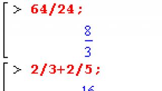
Common fractions are specified using the operation of dividing two integers.
|
|
Note that Maple will automatically reduce fractions. You can perform all basic arithmetic operations on ordinary fractions. If, when specifying a fraction, its denominator is reduced, then such a “fraction” is interpreted by the Maple program as an integer. To convert a fraction to a decimal use the command evalf(). The second parameter of this command specifies the number of significant digits. Note that the decimal representation is just an approximation of the exact value represented by a fraction, i.e. a fraction and its decimal representation are not identical Maple objects. |

Radicals are specified as the result of raising integer or fractional numbers to a fractional power, or calculating the square root of them with the function sqrt(), or root n-th power function surd(number, n).
Floating point numbers are specified as integer and fractional parts separated by a decimal point. They can also be represented using the so-called exponential notation (the symbol is used to indicate the order e or E).
Constants
Maple contains a number of predefined named constants- those whose values can be accessed by name. Some of these constants cannot be changed. These include:
Number e is given as exp(1).
You can view all the constants defined in Maple by running the command: ?ininame
In addition to the constants listed on the Help page, all variables whose names begin with _Env, are Maple system constants by default.
Strings
Strings- any set of characters enclosed in DOUBLE quotes. The length of a line in Maple is practically unlimited and can reach a length of 268,435,439 characters on 32-bit computers.
Variables, unknowns and expressions
Each variable Maple has a name that represents a sequence of Latin characters starting with a letter, with lowercase and uppercase letters considered distinct. In addition to letters, variable names can use numbers and underscores, but the FIRST character of the name must be a LETTER.
Expression is a combination of variable names, numbers, and possibly other Maple objects, connected by valid operation signs.
unknown quantity , and an expression containing unknowns is called symbolic expression. It is precisely for working with such expressions that Maple was primarily developed.
An important operation in Maple associated with expressions is the operation assignments (:=). It has the following syntax: variable:= expression; Here, the left side specifies the name of the variable, and the right side specifies any expression, which can be numeric, symbolic, or just another variable.
Variables allow you to store and process various types of data. By default, the Maple variable is of type symbol, representing a symbolic variable, and its value is its own name. When you assign a value to a variable, its type changes to the type of the value assigned to it.
Internal structure of Maple objects
Each algebraic expression is stored by the Maple system in the form of a tree structure, thereby providing access to any of its members or subexpressions, as well as allowing various symbolic transformations to be performed on them. In this structure's representation, each Maple object is divided into first-level subobjects, which in turn are further divided into subobjects, and so on.
Commands that allow you to select parts of objects:
|
rhs(eq) |
Selecting the right side of an equation (or the end of a range) |
|
lhs(equation) |
Selecting the left side of an equation (or the beginning of a range) |
|
number(fraction) |
Isolating the numerator of a numerical or algebraic fraction |
|
denum(fraction) |
Isolating the denominator of a numeric or algebraic fraction |
|
nops(expr) |
Determines the number of operands in an expression |
|
op(exp) op(n,exp) |
Returns the operands of an expression as a list, Retrieves the nth operand of the expression |
|
select(b f, exp) |
true |
|
remove(b f, exp) |
Identifies the operands in an expression for which the Boolean function produces a value false |
|
indets(expr, type) |
Selects subexpressions of a given type in an expression ("*", "+" ...) |
Let's take a closer look at these commands.
An equation is represented as two expressions connected by an equal sign. It should not be confused with the assignment operator (:=). Equation is a Maple object and is used to define real equations. It can be used on the right side of an assignment operation, thereby naming an equation.
In function has() You can specify multiple subexpressions as a list. Its result will be TRUE if and only if at least one of the subexpressions in the list is found.
Type Substitution and Conversion
When performing mathematical transformations, it is often necessary to replace variables in an expression, function, equation, etc., that is, instead of some variable, substitute its representation through some other variables. And sometimes it is necessary to convert an expression from one type to another. (This type conversion may be required to execute some commands that do not work on the original type of expression.) There are several commands in Maple for these purposes:
|
subs(substitution, EXPRESSION) |
Syntactic substitution of one expression for another in EXPRESSION |
|
algsubs(substitution, EXPRESSION) |
Algebraic substitution of one expression for another in EXPRESSION |
|
subsop(N=new value, EXPRESSION) |
Substituting a new value for the Nth operand of an EXPRESSION |
|
convert(EXPRESSION, type) |
Converts an EXPRESSION to a new data type |
|
whattype(EXPRESSION) |
Defines the type of the expression. |
To substitute another expression instead of some variable (expression), use the command subs(), the syntax of which is as follows: subs(old expression=new expression, EXPRESSION) subs(s1, s2, .. sn, EXPRESSION) subs(, EXPRESSION) where is each s1,..sn is the equation defining the substitution.
The first form of the command analyzes EXPRESSION, defines all occurrences of it old expression and substitutes in their place new expression.
The second form of the command allows you to perform a series of substitutions in EXPRESSION, and the substitutions are performed sequentially, starting from s1. This means that after performing the first substitution defined s1, Maple finds occurrences of the left side of the equation s2 in the newly obtained expression and replaces each such occurrence with the expression given on the right side of the equation s2.
That is, occurrences of expressions specified on the left sides of the equations s1, s2, are defined in the initial parameter EXPRESSION. (see examples)
Use the command simplify(), specifying the required replacement as a parameter (see the next section).
Use the command algsubs(), which performs algebraic substitution.
Note that the “old” variable is completely excluded only when using the first of these methods. In other cases, the “old” variable still remains in the transformed expression.
10. PROGRAMMING IN THE ENVIRONMENTMAPLE
The Maple mathematics package allows users to write their own programs, procedures, and libraries. To do this, the package contains a fairly wide range of commands and constructs similar to high-level algorithmic programming languages.
10.1. Conditional operator
Conditional statement in Maple starts with a reserved word if and must necessarily end with a word fi and has the following structure:
if condition then expression 1 else expression 2 fi ;
This construction makes it possible, depending on the value of a logical condition, to execute expression 1 (if the condition is true) or expression 2 (if the condition is false). Expressions 1 or 2 can be any sequence of commands from the Maple package. The conditional operator can be written in abbreviated form:
if condition then expression 1 fi ;
[> restart;
[> x:=4;
x:=4
[>if x>4 then print ('x>4'); else x:=x^2;
print(2*x); fi;
32
To implement complex conditions, it is necessary to use the full version of the conditional operator, which has the following structure.
if condition 1 then expression 1 elif condition2 then expression2... elif condition n then expression n else expression n +1 fi ;
As follows from the structure of this operator, the nesting of conditions can be practically unlimited and is implemented using a service word elif . Any sequence of Maple commands can be used as expressions.
[> restart;
[>x:=8:
[>if x
x:=c
10. 2 . Loop statements
In the Maple mathematical package, four types of loop operators are used to implement a cyclic computational process. The body of all loop operators is a sequence of commands enclosed between service words do And od . The loop operator of an enumerated type, which is contained in almost all algorithmic languages, has the following structure:
for loop variable name from initial value of loop variable by loop variable increment step to final value of loop variable
[>for i from 0 by 4 to 8 do i od;
0
4
8
The while loop operator in Maple looks like
while condition do expression od ;
In this case, the body of the loop (expression) is executed as long as the value of the logical condition is true and terminates if the condition is false.
[> restart;
[>n:=0:
[>while n
1
2
9
The next loop operator is a symbiosis of the two previous ones and has the following structure:
for loop variable name from initial value of loop variable by step increment value while condition do expressions od ;
In this loop statement, expressions are executed as long as the Boolean condition expression is true and the loop variable changes from its initial value in a given increment.
[> restart;
[> for y from 0 by 2 while y
0
2
4
6
The fourth loop operator is designed to work with analytical expressions and is represented by the following structure:
for loop variable name in expression 1 do expression 2 od ;
Here the body of the loop, expression 2, is executed if the symbolic variable specified by its name sequentially takes the value of each of the operands of algebraic expression 1. Note that the operation of this construction depends on the internal representation of expression 1. So, if expression 1 is a sum, then the name of the variable the cycle takes the value of each term in turn, and if the product is a product, then each factor.
[> restart;
[> a:=5*x^2+x+6/x;
[> b:=simplify(%);
![]()
[> for m in a do m; od;
[> for m in b do m; od;
10.3. Function procedures
Function procedures in Maple can be defined in two ways. To specify function procedures, the first method uses the symbol ( ) and is given by the following structure:
function name:=(list of formal parameters) expression;
where the function name is specified by a set of Latin characters, the list of formal parameters is entered separated by commas. An expression is a Maple command that implements the body of a function procedure.
[> f1:=(x1,x2)->simplify(x1^2+x2^2);
[> f 1 (cos(x),sin(x));
1
The second way to specify function procedures is using the command unapply and has the following structure:
function name:= unapply (expression or operation, list of variables);
This method of specifying function procedures is useful when defining a new function through a known one or when the evaluated expression is intended to be used as a function.
Example .
[> f3:=unapply(diff(z(r)^2,r)-2,z);

[ > f3(sin);
[ > combine(%);
10.4. Procedures
Any procedure in Maple begins with a header, consisting of the procedure name, followed by an assignment character and a function word proc , then the formal parameters are indicated in parentheses separated by commas. The procedure must end with a service word end . All expressions and commands are enclosed between function words proc And end constitute the body of the procedure.
procedure name:= proc (list of formal parameters); commands (or expressions); end ;
If a procedure is loaded, it is called by name. The default return value is the value of the last executed statement (command) from the body of the procedure, and the type of result of the procedure depends on the type of the return value.
[> f:=proc(x,y);x^2+y^2;simplify(%);end:
[ > f(sin(x),cos(x));
1
When writing procedures in Maple, you can use a number of commands and service words, in addition to the required minimum set indicated above, which allow you to describe variables, control the exit from the procedure, and report errors.
When describing the formal parameters of a procedure, you can explicitly specify their type using a colon. With this description, Maple automatically checks the type of the actual parameter and issues an error message if it does not match the type of the formal parameter.
The procedure title may be followed by a descriptive part of the procedure, separated from it by a space. When describing local variables used only within a given procedure, you can use a descriptor, which is specified by the service word local , after which you must specify the names of local variables separated by a space. The use of global variables in a procedure can be specified using a function word global , which should be placed in the descriptive part of the procedure.
To exit a procedure anywhere in its body and assign the result of its work to execute the desired command, you can use the command RETURN ( val ), Where val – a return value that can have a different type when exiting from different places in the procedure.
To exit the procedure in an emergency if an error occurs and report the incident, you can use the command ERROR (‘ string ’) , Here string – a message that is displayed on the monitor screen in an emergency situation. Thus, the general view of the procedure structure can be depicted as follows:
procedure name:= proc (list of procedure parameters) local list of local variables, separated by commas; global list global variables separated by commas; RETURN ( val ); ERROR (‘ error in body of procedure ’);… end ;
[>
[ > examp(-1);
[> examp(0);
[ >examp(2);
11. METHODS OF INPUT AND OUTPUT INFORMATION
IN THE ENVIRONMENTMAPLE
To save the names (identifiers) of variables and their values to external memory in the form of a file with the name name . txt you need to enter the command:
save list of variable names separated by commas, “file name with extension txt ”;
If the extension is the character m , then the file will be written in the internal Maple format, with all other extensions in text format. To display the information saved in the file, use the command
read “ file name ”;
[> restart;
[> examp:=proc(x) local y,w; global z; if x
[ > examp(-1);
[> examp(0);
Error, (in examp) Variablex = 0
[ >examp(2);
[ > read "nnn.txt";
You can use the following two commands to record the entire screen content to a file.
First team
writeto ("file name")
As a result of executing this command, all information contained on the screen will be saved in a file with the specified name. Moreover, if the specified file existed in external memory, then the stored information will be replaced with new one.
Second team
appendto ("file name")
allows you to add on-screen information after a given command to the end of an existing file.
[ > f:=12;
[> f1:=factor (y^2-3*y); save f,f1, "n1.txt";
[> appendto("n1.txt");
[> solve(x^2-3*x+2=0,x);
As a result of executing the command save f , f 1, " n 1. txt "; a text file will be created n 1. txt , which will contain the following information:
f:= 12;
f1:= y*(y-3);
and as a result of executing the command appendto (" n 1. txt "); the contents of the file will look like:
f:= 12;
f1:= y*(y-3);
[ > solve ( x ^2-3* x +2=0, x );
2, 1
The Maple package provides a number of commands for displaying information on the screen. The simplest of them are the commands
print (list Maple
lprint (list Maple -expressions separated by commas);
Moreover, if nothing is assigned to a variable, then its name is printed, otherwise its value is printed.
[> x:=y^2: print (x, "primer 1", y, factor(x-5*y));
![]()
[> x:=y^2: lprint (x, "primer 2", y, factor(x-5*y));
y^2, primer 2, y, y*(y-5)
From the above examples it follows that the command print displays comma-separated expressions in natural mathematical form, and the command lprint outputs information in output line style and expressions are separated by commas and spaces.
The Maple package can be used to analyze and graphically interpret numerical information contained in a text file, obtained both using the package itself and other software applications. As a rule, numbers are written line by line in a text file. To read numeric information from a text file, you can use the command:
readdata (“filename”, variable type( integer / float – the last type is set by default), number counter);
Before using this command, you must activate it using the command:
readlib(readdata):
[> restart;
[> readlib(readdata):
[> ff:=readdata("aa.txt",integer,8);
[ > x:=ff;
[ > y:=x;
[ > y1:=ff;
[ > f:=readline("aa.txt");
![]()
Double indexing in a variable ff is due to the fact that numbers are represented as a two-dimensional array, with the number of rows in the array corresponding to the number of rows read, and the number of columns is determined by the last parameter of the command readdata . As follows from the example given, the command readline outputs numeric data as a type variable string .
12. USING THE MATH PACKAGEMAPLEFOR SCIENTIFIC RESEARCH
In this section, we will consider an example of research using Maple for solving applied engineering problems. The given examples show the capabilities of the Maple package in solving engineering problems related to the study of equipment operating modes, depending on the design and technological parameters of complexes, and illustrate the capabilities of the software and command modes of user operation in the Maple environment. The following are excerpts from the research, accompanied by brief explanations.
12.1. Study of the influence of variable parameters of a flat grinding chamber of a countercurrent mill on the speed of the energy carrier
12 .1.1. Formulation of the problem
Jet mills are a type of impact grinders and consist of an accelerating apparatus (one or more), in which a jet of energy carrier gas imparts speed to the particles of the processed material, and a chamber in which the material flows interact with each other and (or) with special impact surfaces. Air is most often used as an energy carrier in jet mills, and less often - inert gas, water vapor, and combustion products.
Jet grinding makes it possible to combine grinding and separation with mixing, drying and other technological processes. And closed-cycle operation ensures minimal dust release into the environment.
Any jet apparatus includes an ejector, which is a unit in which the mixing and exchange of energy of two flows (main and ejected) occurs, and a grinding chamber in which the mixed flows interact. Particles accelerated by the energy carrier in the accelerating tubes of the ejectors enter the grinding chamber, and then into the jet meeting zone (Fig. 12.1.).
The jet emerging from the accelerating tube does not immediately fill the entire cross-section of the grinding chamber; the jet at the point of entry into it breaks away from the walls and then moves in the form of a free jet, separated from the rest of the medium by the interface. The interface is unstable, vortices appear on it, as a result of which the jet mixes with the environment.
When the jet flows out of the accelerating tube, the flow velocity in its outlet section 1-1 at all points of the section are equal to each other. Over the length – the initial section, the axial velocity is constant in magnitude and is equal to the velocity at the section of the accelerating tube V 0 . In the triangle area ABC (Fig. 12.1.) at all points of the jet the velocities of the energy carrier are equal to each other and also equal V 0 - this area forms the so-called core of the jet. Further, the axial speed gradually decreases and in the main section of the long l basic axial speed V OS V 0 .

Rice. 12.1. Scheme of the jet in the grinding chamber
It is known that the speed of the energy carrier from the cutoff of the accelerating tube to the jet collision plane varies according to the law
 ,
(12.1)
,
(12.1)
Where V z – speed of the energy carrier from the grinding chamber at a distance z from the cut of the acceleration tube, m/s;
V 0 – speed of the energy carrier at the exit of the accelerating tube, m/s;
z 0 – distance from the cut of the accelerating tube to the jet meeting plane, m.
When determining the change in the kinetic energy of a finite volume of a continuous medium, it is necessary to know the work of the forces of intercomponent interaction between particles of crushed material and the energy carrier. This work depends on the force vector of the dynamic impact of the energy carrier on the particle, which is calculated as follows
 ,
(12.2)
,
(12.2)
Where R – vector of the force of the dynamic action of air on the particle, N;
F m – cross-sectional area of the particle, m2;
 ,
(12,3)
,
(12,3)
Let's denote
 ,
(12.8)
,
(12.8)
Where m – mass of particle of crushed material, kg.
 ,
(12.9)
,
(12.9)
Where  - particle density of the crushed material, kg/m.
Expression (12.7) will take the form
 .
(12.10)
.
(12.10)
The resulting equation can be used to determine the change in the speed of particles of the ground material in the grinding chamber from the cut of the accelerating tubes to the area of interaction of counter flows.
A system of differential equations describing the process of changing the speed of particles and energy carriers in the grinding chamber from the cut of the accelerating tube to the area of collision of oncoming flows
 .
(12.11)
.
(12.11)
Distance l page – between the cut of the accelerating tube and the middle plane in the grinding chamber is selected from the condition
Where d tr = 18 acceleration tube diameter, mm.
Department: Information Technologies
Laboratory work
On the topic of: " SYNTAX, MAIN OBJECTS AND SYSTEM COMMANDS MAPLE "
Moscow, 2008
Goals of work :
· know the main objects and variables of the Maple system;
· know and be able to apply commands used when working with objects and variables of the Maple system;
· know the syntax of the basic mathematical functions of the Maple system.
Introduction
Maple Analytical Computing System is an interactive system. In this case, this means that the user enters a command or Maple language operator in the worksheet input area and, by pressing the key
Each operator or command Necessarily are completed separator sign. There are two such characters in the Maple system - semicolon (;) and colon (:). If the clause ends with a semicolon, it is evaluated and the result is displayed in the output area. When you use a colon as a delimiter, the command runs, but the results are not displayed in the worksheet output area. This is convenient, for example, when programming in Maple, when there is no need to output any intermediate results obtained from loop operators, since the output of these results can take up a lot of space on the worksheet, and it can take a significant amount of time to display them.
Here and below, Maple commands are written in the syntax form of the Maple language. If, when executing examples, there is a desire to display commands in mathematical notation, then follow the command Options ® Input Display ® Standard Math Notation set the appropriate display mode.
Maple implements its own language through which the user communicates with the system. The basic concepts are objects and variables, from which expressions are constructed using valid mathematical operations.
The simplest objects, with which it can work Maple , are numbers, constants and strings.
Numbers
Numbers in the Maple system can be of the following types: integers, fractions, radicals, floating point numbers, and complex numbers. The first three types of numbers allow you to perform precise calculations (without rounding) of various mathematical expressions, implementing exact arithmetic. Floating point numbers are approximate numbers in which the number of significant digits is limited. These numbers serve to approximate (or approximate) the exact Maple numbers. Complex numbers can be either exact, if the real and imaginary parts are represented by exact numbers, or approximate, if floating point numbers are used to specify the real and imaginary parts of a complex number.
Whole numbers are given as a sequence of numbers from 0 to 9. Negative numbers are given with a minus sign (–) in front of the number; zeros before the first non-zero digit are not significant and do not affect the value of the integer. The Maple system can work with integers of arbitrary size; the number of digits is practically limited to 2 28. Calculations with integers implement four arithmetic operations (addition +, subtraction –, multiplication *, division /) and factorial calculation (!).
Maple represents a large integer that does not fit on the output line by using the backslash character (\) as the output continuation character on the next line. The last command calculates the number of digits from the previous calculation. It uses the % operation as a parameter, which is just a convenient form of reference to the result of the previous operation. Maple has two other similar operations that identify the results of the preprevious and preprevious commands. Their syntax is, respectively, as follows:
Maple has a fairly large set of commands that allow you to perform actions specific to the processing of integers: factorization into prime factors (ifactor), calculation of the quotient (iquo) and remainder (irem) when performing an integer division operation, finding the greatest common divisor of two integers ( igcd), perform a check to see if an integer is prime, and much more.
To check the calculation of the quotient and remainder of two integers, the operations of obtaining the result of executing the previous (calculating the quotient) and the previous (calculating the remainder) commands were used. The result of the isprime() command is a Boolean constant true or false.
By typing a command in the worksheet input area? integer, you can get a list of all commands for working with integers
Common fractions are specified using the operation of dividing two whole numbers. Note that Maple automatically performs the fraction reduction operation. You can perform all basic arithmetic operations on ordinary fractions.
If, when specifying a fraction, its denominator is reduced (see the last calculation in the example), then such a “fraction” is interpreted by the Maple system as an integer.
Often presenting a result as a fraction is not very convenient, and the problem arises of converting it to a decimal fraction. To do this, use the evalf() command, which approximates a common fraction with floating point numbers using ten significant digits in the mantissa of their representation. If the default accuracy is not sufficient, then it can be set as the second parameter of the specified function.
A fraction and its decimal representation are not identical Maple objects. Decimal notation is just approximation exact value represented by an ordinary fraction.
Radicals are specified as the result of raising integer or fractional numbers to a fractional power, or calculating the square root of them using the sqrt() function, or calculating the root n-th power using the surd(number, n) function. The operation of exponentiation is specified by the symbol ^ or a sequence of two asterisks (**). When raising fractions to powers, they should be enclosed in parentheses, just like the fractional exponent. When specifying radicals, possible simplifications are also made related to removing the maximum possible value from under the sign of the radical.
Calculations with integers, fractions and radicals are absolutely accurate, because Maple does not perform any rounding when working with these data types, unlike floating point numbers.
Floating point numbers are specified as integer and fractional parts separated by a decimal point, preceded by a number sign, for example, 3.4567, -3.415. Floating-point numbers can be written using what is known as exponential notation, in which the symbol e or e is placed immediately after a real floating-point number or a regular integer called the mantissa, followed by a signed integer (exponent). This form of notation means that the mantissa must be multiplied by ten to the power of the number corresponding to the exponent to obtain the value of the number written in this exponential form. For example, 2.345e4 corresponds to the number 23450.0. Thus, it is possible to represent numbers that are very large in absolute value (the exponent is a positive number) or very small (the exponent is a negative number).
Mathematical expressions are constructed from numbers using arithmetic operations. The symbols for arithmetic operations in Maple are listed in Table. 1.
Table 1. Arithmetic operations
The sequence of arithmetic operations follows the standard rules of precedence of operations in mathematics: first exponentiation is performed, then multiplication and division, and finally addition and subtraction. All actions are performed from left to right. The factorial calculation operation has the highest priority. To change the sequence of arithmetic operations, use parentheses.
If all numbers in an expression are integers, fractions, or radicals, then the result is also represented using these data types, but if there is a floating point number in the expression, then the result of evaluating such a “mixed” expression will also be a floating point number, unless there is no radical present in the expression. In this case, the radical is calculated exactly, and its coefficient is calculated either exactly or as a floating point number, depending on the type of factors.
Maple's analytical calculation system always attempts to produce calculations with absolute accuracy. If this does not work, then arithmetic with real numbers is used.
Maple can also work with complex numbers . For an imaginary unit
Maple uses a constant I. The assignment of a complex number is no different from its usual assignment in mathematics.
SOLVING MATHEMATICAL PROBLEMS
IN MAPLE
PART I
FEDERAL AGENCY FOR EDUCATION
State educational institution of higher education
"Nizhny Novgorod State University named after. »
MATHEMATICAL PROBLEMS IN MAPLE
faculty for students studying
direction of preparation 010100 - “Mathematics”.
Nizhny Novgorod
UDC 621.396.218
Solving problems in MAPLE. Part I. Compiled by: , : Educational and methodological development. – N. Novgorod: Nizhny Novgorod State University Publishing House, 2007. – 35 p.
Reviewers:
Associate Professor of the Department of Chifa, Faculty of Computational Mathematics and Mathematics,
Ph.D. n. ,
Associate Professor of the Department of Education and Science, Faculty of Physics,
This development is a practical guide to exploring the capabilities of the analytical calculation package Maple. Consistent study of topics and completion of assignments will allow you to master, step by step, the basic techniques of working in a mathematical system Maple.
The educational and methodological development is intended for 2nd and 3rd year students of the Faculty of Mechanics and Mathematics.
UDC 621.396.218
© Nizhny Novgorod State
University named after , 2007
Computer algebra systems are new technologies in scientific research and education. In recent years, general-purpose systems such as Maple and Mathematica have become widespread.
The Maple system is included in the integrated Scientific WorkPlace system and is used in many leading universities around the world both in scientific research and in the educational process. The Maple core is included in other common packages such as MathCad, MathLab.
This development will allow a beginner to enter the technology of using the Maple system, gain first skills, after which he will be able to independently understand the more subtle issues of using Maple. I would like to note that this development is in no way a description of the Maple system. It is intended primarily to teach math students how to solve basic math problems using Maple.
1. INITIAL INFORMATION. DATA TYPES
The dialogue with the system proceeds in a “question-answer” style. The command starts with a symbol > and ends with either a comma ( ; ), or a colon ( : ). To execute a command you must press the key Enter. If there is a semicolon at the end of the command, the result of the command or an error message will be displayed on the screen. A colon at the end of the command means that the command will be executed, but its result will not be displayed on the screen. Symbol # used to enter text comments. You can also use the T key on the toolbar to enter text. To return to entering commands, press the key with the > symbol. To call the result of previous commands, use the symbols %, %% or %%%, respectively. Team restart cancels the result of all previous commands.
Variables in Maple are characterized by a name and a type. A variable name in Maple can consist of letters, numbers and some special characters, but must begin with a letter. There are no restrictions on name length. In addition, Maple distinguishes between lowercase and uppercase letters. To assign a specific value to a variable, use the operator := . Variables can be used in mathematical expressions and functions without being previously defined.
Let's look at the features of writing data of numeric, string and multiple types in Maple.
The expression belongs to the integer type ( integer), if it consists of a sequence of numbers not separated by any characters. Expressions of the form a/b, where a, b are integers, belong to the fractional type ( fraction). To floating point numbers ( float) include expressions of the form a. b, a. And. b. Also numbers like float can be written in exponential form a*10^b. Complex numbers ( complex) in Maple are written in algebraic form: a+I*b, where a, b are real numbers.
String expression type string is any finite sequence of characters enclosed on both sides by upper double quotes. A sequence of characters enclosed in backquotes is considered to be the character ( symbol).
A bunch of ( set) in Maple is specified by listing the elements of the set in curly braces. For example,
> A:=(x^n$n=1..6);
> B:=(a, a,b, b,b, c);
https://pandia.ru/text/78/155/images/image003_72.gif" width="197" height="26">
To create an array, use the command array(i1..j1, i2..j2,..., M), which returns an array with elements from the list M.
Elements of a set, list, or array are accessed by indicating the element indices in square brackets.
> V:=array(1..2,1..2,1..2,[[,],[,]]);
 https://pandia.ru/text/78/155/images/image006_53.gif" width="16 height=19" height="19">
An array can also be specified with a command like V:=array(1..2,1..2,1..2,); , then redefining the values of V using the assignment operator.
In Maple you can write the letters of the Greek alphabet in printed form. To do this, type the name of the Greek letter on the command line.
> beta+Gamma+delta;
Task 1.1
1. Define a set A consisting of integers from 3 to 20, and a set B consisting of the squares of these numbers. Find the union, intersection, difference of sets A and B. Find the powers of all resulting sets.
2. Define a custom list and a four-dimensional array.
2. ARITHMETIC OPERATIONS, FUNCTIONS. ARITHMETIC CONVERSIONS
EXPRESSIONS AND SOLVING EQUATIONS
2.1. Calculations in Maple
To write mathematical expressions in Maple, the addition (+), subtraction (-), multiplication (*), division (/), exponentiation (^) and assignment operators (:=) are used. The order in which mathematical operations are performed is standard.
Example.
> (a*b^4-(a*b)^4)/7;

Basic constants in Maple are denoted as follows: Pi- number π, I- imaginary unit i, exp(1)- base of natural logarithms e, infinity- infinity, true- truth, false- lie. The following comparison signs are used: <, >, >=,<=, <>, = .
The Maple system copes equally well with both symbolic and numerical calculations. By default, calculations are carried out symbolically.
Example.
>1/2+123/100+ sqrt(3);
The part of the expression that contains a floating point number (float) will be calculated approximately.
Example.
>2+ sqrt(2.0)- Pi;
All calculations are carried out to ten significant figures by default. The number of significant digits can be changed using the command > Digits: = n.
In order to obtain the value of an expression in numerical form, use the function
https://pandia.ru/text/78/155/images/image012_43.gif" width="414" height="19">
2.2. Setting functions
Maple has a large number of functions built-in. Let us list the notation for the main elementary functions..gif" width="83 height=57" height="57">
Let's look at several ways to define new functions:
1) assignment to a variable of some expression
variable name:=expression;
variable name(parameter list):=expression;
Example.
> f(t):= cos(t)^2+1;
![]()
> f(0);
With this method of specifying a function, in order to calculate the value of the function at a certain point, you need to determine the values of variables (parameters) using the assignment operator, or use the substitution operator subs.
https://pandia.ru/text/78/155/images/image018_28.gif" width="106" height="33">
> value(%);
https://pandia.ru/text/78/155/images/image021_25.gif" width="100" height="33">
>x:= Pi: y:=10: f;
Team value(expression) used to evaluate the value of an expression.
It should be noted that after assigning the variable x a specific value x:=a, the variable x will no longer be undefined. You can return x to the status of an undefined variable with the command > x:= evaln(x); or remove the assignment with the command > x:=’ x’ ; or cancel all assignments with the command restart.
2) Defining a function using a function operator
function name:=parameter list-> expression;
A function defined in this way is accessed in the standard way: function name(a, b, ...), where a, b, ... are specific variable values.
Example.
> f1:=(x, y, z) -> x^(y^ z);
![]()
> f1(2,2,2); f1(x,2,2);
https://pandia.ru/text/78/155/images/image024_25.gif" width="25" height="26 src=">
3) The function can be set using the command
unapply(expression, parameters), which converts the expression into a function operator.
Example.
> f2:=unapply(sin(x)^2+2*exp(y^2),x, y);
> f2(Pi/4,1);
https://pandia.ru/text/78/155/images/image027_22.gif" width="189" height="107"> the command is used
https://pandia.ru/text/78/155/images/image028_21.gif" width="248" height="77">
> f1:=convert(f, piecewise);

> f2:=unapply(f1,x);
> f2(-1/2); f2(-1);
https://pandia.ru/text/78/155/images/image032_20.gif" width="196" height="27">.gif" width="73" height="49">. Simplify the resulting expressions.
3. Find the meaning of the expression ![]() . To perform complex number transformations, use the function evalc.
. To perform complex number transformations, use the function evalc.
4. Write the function ![]() without modulus sign.
without modulus sign.
5. Set  and find f(-10)+3f(-1)+f(3).
6. Set the function  as a functional operator and find its value at x=-1, y=.
2.3. Converting Math Expressions
Maple has extensive capabilities for analytical transformations of mathematical formulas. These include operations such as bringing similar ones, factoring, opening parentheses, reducing a rational fraction to normal form, and many others.
In Maple you can transform both the entire expression and its individual parts.
To select the left (right) part in a mathematical expression of the form A=B, use the commands
lhs(expression);
rhs(expression);
To select the numerator (denominator), use the commands
number(expression);
denom(expression);
Example.
>F:=(a^3+b)/(a-b)=3*a^2+b^2/(a+b);

>numer(rhs(F));
![]()
>denom(rhs(F));
To select some part of an expression, list or set, use the command
op(i,expression), where i is a number that determines the position in the expression.
Example.
> x+ y+ z; >op(2,%);
Gif" width="12" height="12 src="> isolate(equation, expression);
Example.
> P:= 2* ln(x)* exp(x) -3* exp(y)+7=10* ln(x) - exp(y):
> isolate(P, y);

> R:=5*(x^2)*sin(x)+1=5*sin(x):
> isolate(R, sin(x));

1) Reduction of similar terms in an expression for a variable is carried out by the command
https://pandia.ru/text/78/155/images/image047_14.gif" width="439" height="28">
2) You can factor the expression using the command
https://pandia.ru/text/78/155/images/image050_16.gif" width="186" height="56">
>factor(x^4-3*x^3+2*x^2+3*x-9);
>factor(x^3+x-3*sqrt(2));
>factor(x^3+16, (2^(1/3),sqrt(3)));
>alias(w=RootOf(x^3+2*x+1)); factor(x^3+2*x+1,w);
https://pandia.ru/text/78/155/images/image055_15.gif" width="504" height="26 src=">
> convert(%,radical);
https://pandia.ru/text/78/155/images/image057_17.gif" width="303" height="57">
> factor(x^2+x+1,complex);
Gif" width="12" height="12 src="> expand(expression, options), where in the options you can specify an expression whose parenthesis should not be expanded. This command is also used to manipulate exponents and reduce trigonometric expressions to trigonometric functions of simple arguments.
Example.
>expand((x+1)*(x+2)*(x+3)*(x+4));
>expand((x+y)*(x+3), x+3);
>expand(exp(a-n*b+ln(c)));
>expand(tan(3* x));

4) You can bring a fraction to normal form using the command
https://pandia.ru/text/78/155/images/image063_16.gif" width="60" height="54">
>normal(sin(2*x+3+4/(x-1)+5/(x-2)), expanded);

5) To transform expressions containing radicals, use the command
rationalized" in order to get rid of irrationality in the denominators, " expanded" to expand all parentheses.
Example.
> (7+5* sqrt(2))^(1/3);
![]()
> radnormal((7+5* sqrt(2))^(1/3));
> a := sqrt(3)/(3^(1/2)+6^(1/2));
rationalized");
6) Simplification of expressions is carried out by the command
DIV_ADBLOCK515">
Example.
>(sqrt(2)+sqrt(3))*(sqrt(2)-sqrt(3));
>simplify((sqrt(2)+sqrt(3))*(sqrt(2)-sqrt(3)));
> f:=(1-cos(x)^2+sin(x)*cos(x))/(sin(x)*cos(x)+cos(x)^2); simplify(f, trig);

The options also specify assumptions about the value of the argument. For formal symbolic transformations of multi-valued functions, you can specify in the options symbolic.
Example.
> g:=sqrt(x^2);
> simplify(g, assume=real);
> simplify(g, assume=positive);
>simplify(g, symbolic);
The simplify command allows you to perform transformations in an expression under specified conditions (conditions are indicated in curly braces).
Example.
> f:= -3*x*y + x+y: simplify(f, (x = a-b, y = a+b));
![]()
In some cases, it may be useful to pre-convert an expression using the command
https://pandia.ru/text/78/155/images/image076_12.gif" width="276" height="54">
>simplify(B, trig);

>convert(%,tan):
>simplify(%);
7) You can combine parts of an expression according to certain rules using the command
https://pandia.ru/text/78/155/images/image079_12.gif" width="94" height="25 src=">, , when specifying the option ln potentiation occurs. Just like for simplify, you can specify in the options symbolic.
Example.
> combine(exp(sin(a)*cos(b))*exp(-cos(a)*sin(b)),);
>combine((a^3)^2+a^3*a^3);
Gif" width="12" height="12 src="> solve(equation, variables).
Variables are listed in curly braces separated by commas. If you do not specify a set of variables in the command parameters, then the solution will be found for all variables participating in the equations. If you need to solve a system of equations, then the equations of the system are indicated in curly brackets, separated by commas. The result of using the solve command will be a list of solutions to the given equation, or, if the equation has no solutions or they cannot be found by the solve command, no messages will appear in the output line. You can work with a list of solutions in the same way as with a regular list.
Example.
> eq:=(x-1)^3*(x-2)^2;
> s:=solve(eq);
![]()
> solve(x^4-11*x^3+37*x^2-73*x+70);
https://pandia.ru/text/78/155/images/image086_12.gif" width="349" height="22 src=">
>e:=solve(AX);
>rhs(e); subs(e, z);
DIV_ADBLOCK517">
Example.
>e1:=(x^2-y^2=1,x^2+x*y=3);
> s:=solve(e1,(x, y));
> _EnvExplicit:=true:
> solve(e1,(x, y));
The maximum number of solutions that can be found using the solve command is determined by the value of the global variable _MaxSols, which has a default value of 100. If you assign a global variable _EnvAllSolutions meaning true, then in the case of an infinite number of solutions, the solve command for some equations will be able to formulate the answer in the form of an expression containing variables of a certain type. For example, for trigonometric equations, the answer will contain integer parameters of the form _Z~.
Example.
> _EnvAllSolutions:= true:
>solve(sin(2*x)=cos(x), x);
https://pandia.ru/text/78/155/images/image094_11.gif" width="274" height="51 src=">.gif" width="12" height="12 src="> fsolve(equation, variables, options).
In the options you can specify the interval in which the roots will be searched, you can also specify complex - to find all complex roots, or the option maxsols=n– to find the n smallest roots of a polynomial. If the equation is given by a polynomial, then the command fsolve will find all real approximate roots, in general the fsolve command will find only one numerical root of the equation; other roots can be searched by changing the search interval so that the found root is not included in it.
Example.
> fsolve(x-cos(x));
https://pandia.ru/text/78/155/images/image097_10.gif" width="641" height="23">
To resolve recurrences, use the command
https://pandia.ru/text/78/155/images/image098_10.gif" width="255" height="22 src=">
> rsolve(e1,f);
> rsolve((e1,f(0)=1,f(1)=2),f);
The solve command can also be used to solve inequalities and systems of equations and inequalities.
Example.
> solve(ln(x)<1, x);
https://pandia.ru/text/78/155/images/image102_8.gif" width="119" height="23 src=">
> solve((x-y>=1,x-2*y<=1,x-3*y=0,x+y>=1),(x, y));
https://pandia.ru/text/78/155/images/image104_7.gif" width="180" height="56">.
2. Simplify the expression.
3. Simplify the expression.
4.Give similar ones in the expression and calculate its value for a=-3, x=1.
5. Simplify expression a) ![]() ; b)
; b)  .
.
6. Get rid of irrationality in the denominator of the expression.
7. Express, https://pandia.ru/text/78/155/images/image113_7.gif" width="46" height="48 src="> in radicals.
8. Prove that if A, B, C are the angles of a triangle.
9. Express through and https://pandia.ru/text/78/155/images/image118_7.gif" width="164" height="41">;
b) https://pandia.ru/text/78/155/images/image120_7.gif" width="88" height="47 src=">.
11. Expand the polynomial ![]() to factors over the field of real numbers and over the field of rational numbers. Find the expansion in radicals.
to factors over the field of real numbers and over the field of rational numbers. Find the expansion in radicals.
12. Factor the polynomial over the field of real numbers and over the field of complex numbers. Find the expansion in radicals.
13. Solve the equation ![]() .
.
14. Solve the system of equations  .
.
15. Solve the system of equations  and simplify the answer.
16. Numerically find all solutions to the equation ![]() .
.
17. Find three numerical solutions to the equation.
18. Solve the system of inequalities.
19. Solve the inequality.
3 . CONSTRUCTION OF CHARTS
This part is devoted to the capabilities of the Maple V system in visualizing a wide variety of calculations.
3.1. 2D graphs
To plot function graphs f(x) from one variable (in the interval https://pandia.ru/text/78/155/images/image132_6.gif" width="69" height="24"> along the axis OU) command is used
plot(f(x), x=a..b, y=c..d, options),
Where options– an option or set of options that specifies the style of plotting. If they are not specified, the default settings will be used. Image adjustments can also be made from the toolbar. To do this, left-click on the image. After this, the buttons in the bottom row of the panel become active. You can also find out the coordinates of a point on the graph. To do this, move the cursor to the desired point on the graph and click the left mouse button. Coordinates will appear on the left in the bottom row of buttons on the panel. Image settings can also be done using the context menu. It is called with the right mouse button.
Basic command parameters plot:
title=”text”, Where text- title of the figure (text can be left without quotes if it does not contain spaces).
coords=polar – setting polar coordinates (the default is Cartesian).
axes– setting the type of coordinate axes: axes=NORMAL– conventional axles; axes=BOXED– graph in a frame with a scale; axes=FRAME– axis centered in the lower left corner of the figure; axes=NONE– without axles.
scaling– setting the drawing scale: scaling=CONSTRAINED– identical scale along the axes; scaling=UNCONSTRAINED– the graph is scaled to fit the window size.
style= LINE– line output, style= POINT output in dots.
numpoints=n– number of calculated graph points (by default n=50).
сolor– setting line color: English color name, for example, yellow– yellow, etc.
xtickmarks=nx And ytickmarks=ny– number of marks along the axis Oh and axles Oh, respectively.
thickness=n, Where n=1,2,3…- line thickness (default n=1).
linestyle=n– line type: continuous, dotted, etc. (default n=1– continuous).
symbol=s - type of symbol used to mark points: BOX, CROSS, CIRCLE, POINT, DIAMOND.
font=– setting the font type for text output: f sets the name of the fonts: TIMES, COURIER, HELVETICA, SYMBOL; style sets the font style: BOLD, ITALIC, UNDERLINE; size– font size in pt.
labels=– inscriptions along the coordinate axes: tx– along the axis Oh And ty– along the axis Oh.
discount=true– an indication for constructing infinite discontinuities, while asymptotes are not drawn on the graph.
Example. Build a graph https://pandia.ru/text/78/155/images/image134_1.jpg" width="292 height=292" height="292">
Plotting a graph of a function specified parametrically
Using the command plot you can also build graphs of functions specified parametrically y=y(t), x=x(t) :
plot(, parameters).
Example. Draw a graph of a parametric curve, https://pandia.ru/text/78/155/images/image138_2.jpg" width="231 height=164" height="164">
Graphing a Function Defined Implicitly
To plot an implicit function F(x, y)=0 the command is used https://pandia.ru/text/78/155/images/image139_5.gif" width="80" height="27">.
>with(plots):implicitplot(x^2+y^2=1, x=-1..1, y=-1..1);
Gif" width="12 height=12" height="12"> textplot(, options), Where x0, y0– coordinates of the point from which text output begins 'text'.
Displaying several graphic objects on one drawing
If you need to combine several function graphs in one picture, you can use the command
plot((f1(x), f2(x), …), options);
If you need to draw several graphic objects obtained using different commands, then for this the result of the commands is assigned to some variables:
> p:= plot(…): t:= textplot(…):
In this case, no output is produced on the screen. To display graphic images, you need to run the command from the package plots:
display(, options).
Example. Build function graphs https://pandia.ru/text/78/155/images/image142_6.gif" width="73" height="20 src=">.gif" width="59" height="24 src= "> in one picture.
> with(plots):
> p1:=plot(sin(x), x=-5..5, y=-2..2, thickness=3, color=blue):
> p2:=plot(cos(x), x=-5..5, y=-2..2, thickness=3, color=green):
> p3:=plot(tan(x), x=-5..5, y=-2..2, thickness=3, color=black):
> p4:=plot(ln(x), x=-5..5, y=-2..2, thickness=3, color=red):
> display(p1,p2,p3,p4);
https://pandia.ru/text/78/155/images/image146_5.gif" width="297 height=24" height="24"> , then you can use the command for this inequal from the package plots:
inequals((f1(x, y)>c1,…,fn(x, y)>cn), x=x1…x2, y=y1..y2, options)
The system of inequalities defining the area, then the dimensions of the coordinate axes and parameters are indicated in curly brackets. Using the parameters, you can adjust the thickness of border lines, the colors of open and closed borders, and the colors of outer and inner areas:
.gif" width="12" height="12 src=">optionsexcluded=(color=yellow)– setting the color of the outer area;
.gif" width="12" height="12 src=">optionsclosed(color=green, thickness=3)– setting the color and thickness of the closed border line.
Task 3.1
1. Create a graph https://pandia.ru/text/78/155/images/image148_6.gif" width="75" height="43">.
3..gif" width="72" height="20">, framed.
4..gif" width="83" height="23 src=">
> plot(1-sin(x^2), x=0..2*Pi, coords=polar, color=black, thickness=4);
5. Construct a graph of a hyperbola: .
6..gif" width="75" height="20 src=">) inscribed in an ellipse. Label these lines in bold italics.
> with(plots):
> eq:= x^2/16+ y^2/4=1:
> el:=implicitplot(eq, x=-4..4, y=-2..2, scaling=CONSTRAINED, color=green, thickness=3):
> as:=plot(, color=blue, scaling=CONSTRAINED, thickness=2):
> eq1:=convert(eq, string):
> t1:=textplot(, font=, align=RIGHT):
> t2:=textplot(, font=, align=RIGHT):
> t3:=textplot(, font=, align=LEFT):
> display();
7. Construct an area bounded by the lines: , , .
> with(plots):
> inequal((x+y>0, x-y<=1, y=2}, x=-3..3, y=-3..3,
optionsfeasible=(color=red),
optionsopen=(color=blue, thickness=2),
optionsclosed=(color=green, thickness=3),
optionsexcluded=(color=yellow));
3 .2. Three-dimensional graphics. Animation
Graph of a surface defined by an explicit function
A function can be graphed using the command
plot3d(f(x, y), x=x1…x2, y=y1…y2, options).
The options for this command overlap with the options for the plot command. To frequently used command parameters plot3d also applies
light=– setting the illumination of the surface created from a point with spherical coordinates ( angl1, angl2). Color is determined by fractions of red ( c1), green ( c2) and blue ( c3) colors that are in the interval .
style=opt sets the drawing style: POINT–points, LINE– lines, HIDDEN– grid with removal of invisible lines, PATCH– placeholder (set by default), WIREFRAME– grid with invisible lines, CONTOUR– level lines, PATCHCONTOUR– filler and level lines.
shading=opt specifies the filler intensity function, its value is xyz- default, NONE– without coloring.
It is more convenient to customize 3D images without using command options plot3d, but using the program's context menu. To do this, right-click on the image. Then the image adjustment context menu will appear. The commands in this menu allow you to change the image color, backlight modes, set the desired axes type, and line type. Just like for two-dimensional graphs, you can activate the bottom row of buttons on the toolbar by left-clicking on the image. You can rotate the image using the panel buttons or by holding the left mouse button.
Example. Construct a surface along with level lines
https://pandia.ru/text/78/155/images/image160_0.jpg" width="321" height="198">
Graph of a surface defined parametrically
If you need to construct a surface defined parametrically: x=x(u,v), y=y(u,v), z=z(u,v), then these functions are listed in square brackets in the command:
plot3d(, u=u1..u2, v=v1..v2).
Example. Build a torus.
> plot3d(, s=0..2*Pi, t=0..11*Pi/6, grid=, style=patch, axes=frame, scaling=constrained);
https://pandia.ru/text/78/155/images/image162_4.gif" width="99" height="24">, built using the package command plots:
implicitplot3d(F(x, y,z)=c, x=x1..x2, y=y1..y2, z=z1..z2), where the equation of the surface and the dimensions of the pattern along the coordinate axes are indicated.
Spatial curve graph
In the package plots there is a team spacecurve to construct a spatial curve specified parametrically: .
spacecurve([ x(t), y(t), z(t)], t= t1.. t2) , where the variable t varies from t1 before t2.
Plotting multiple 3D shapes on one graph
Team plot3 d allows you to simultaneously build several figures intersecting in space. To do this, instead of describing one surface, it is enough to specify a list of descriptions of a number of surfaces. In this case, the function plot3 d has a unique feature - it automatically calculates the intersection points of shapes and shows only the visible parts of the surfaces. This creates images that look completely natural.
Example. Construct two surfaces and ![]() within https://pandia.ru/text/78/155/images/image168_4.gif" width="39" height="19">.
within https://pandia.ru/text/78/155/images/image168_4.gif" width="39" height="19">.
> plot3 d({ x* sin(2* y)+ y* cos(3* x), sqrt(x^2+ y^2)-7}, x=- Pi.. Pi, y=- Pi.. Pi, grid=, axes= FRAMED, color= x+ y);

Animation
Maple allows you to display moving images on the screen using commands animate(two-dimensional) and animate3d(three-dimensional) from the package plots. The essence of animation when using these functions is to construct a series of frames, with each frame associated with the value of a time-varying variable t. Among the command parameters animate3d There is
frames– number of animation frames (default frames=8).
It is more convenient to control a moving image using the context menu.
Exercise 3 .2
1. Construct a surface graph.
2. Build a ball ![]() :
:
3..gif" width="65" height="21 src=">.gif" width="173 height=53" height="53">.gif" width="95" height="48 src=" >.gif" width="71" height="23 src=">.
Print the name of the picture, label the axes and set the same scale on the axes.
6. Draw a moving object - a Mobius strip.
4 . MATHEMATICAL ANALYSIS
Let's look at the main functions for solving mathematical analysis problems built into the Maple package.
4 .1. Limit of a function and differentiation
Limits are calculated using the command
.gif" width="12" height="12 src="> Limit(expression, x=a, parameters).
Example.
>Limit(ln(cos(a*x))/(ln(cos(b*x))), x=0)=limit(ln(cos(a*x))/(ln(cos(b*x ))), x=0);https://pandia.ru/text/78/155/images/image181_4.gif" width="215" height="58 src=">
Differentiation in Maple is done using the command
DIV_ADBLOCK519">
https://pandia.ru/text/78/155/images/image182_4.gif" width="262" height="54">
IN Maple There are several ways to represent a function.
Method 1: Defining a function using the assignment operator ( := ): a name is assigned to some expression, for example:
> f:=sin(x)+cos(x);
If you set a specific variable value X, then we get the value of the function f for this X. For example, if we continue the previous example and calculate the value f when , then we should write:
> x:=Pi/4;
After executing these commands the variable X has a given value.
In order not to assign a specific value to a variable at all, it is more convenient to use the substitution command subs((x1=a1, x2=a2,…, ),f), where variables are indicated in curly braces xi and their new meanings ai(i=1,2,...), which should be substituted into the function f . For example:
> f:=x*exp(-t);
> subs((x=2,t=1),f);
All calculations in Maple by default are produced symbolically, that is, the result will explicitly contain irrational constants such as, and others. To get an approximate value as a floating point number, use the command evalf(expr,t), Where expr- expression, t– accuracy expressed in numbers after the decimal point. For example, in continuation of the previous example, let’s calculate the resulting function value approximately:
> evalf(%);
The symbol used here is ( % ) to call the previous command.
Method 2: Defining a function using a function operator that maps to a set of variables (x1,x2,…) one or more expressions (f1,f2,…). For example, defining a function of two variables using a function operator looks like this:
> f:=(x,y)->sin(x+y);
This function is accessed in the most familiar way in mathematics, when specific values of variables are indicated in parentheses instead of function arguments. Continuing the previous example, the value of the function is calculated:
Method 3: Using a command unapply(expr,x1,x2,…), Where expr- expression, x1,x2,…– a set of variables on which it depends, you can transform the expression expr into a functional operator. For example:
> f:=unapply(x^2+y^2,x,y);
![]()
IN Maple it is possible to define non-elementary functions of the form

via command
> piecewise(cond_1,f1, cond_2, f2, …).
For example, the function

is written as follows.