The most convenient way to calculate and work with percentages is in Excel in the Microsoft Office package, because all that is required is to enter the values and the desired formula.
A percentage is a hundredth of a whole number, which on paper is indicated by the sign% or decimal fractions (70% \u003d 0.70). The standard expression for percentage calculations is Whole/Part*100, but thanks to Excel, you don't have to manually calculate anything.
How to calculate percentages in Excel
The simplicity of working with the program lies in the fact that it is enough for the user to enter the values of the whole and its parts (or select from the previously entered data), and indicate the principle of calculation, and Excel will perform the calculations on its own. In Excel, the percentage is calculated like this − Part/Whole = Percentage, and multiplication by 100 happens automatically when the user selects the percentage format:

For calculations, let's take the calculation of the implementation of the work plan:


The program will independently calculate the percentage of plan completion for each product.
Percentage of the number
In Excel, you can calculate a number, knowing only its fraction: %*Part = Integer. Let's say you need to calculate what is 7% of 70. To do this:

If the calculation is carried out when working with a table, then instead of entering numbers, you must give links to the desired cells. It is worth being careful, when calculating the format should be General.
Percentage of the amount

If the data is scattered throughout the table, then you need to use the formula SUMIF- it adds up the values that meet the given parameters, in the example - the given products. An example formula would look like this - “=SUMIF (criteria range; addition range) / total amount”:

Thus, each parameter is considered, i.e. product.
Calculating percentage change
Comparing two shares is also possible using Excel. To do this, you can simply find the values \u200b\u200band subtract them (from the larger to the smaller), or you can use the increase / decrease formula. If you need to compare the numbers A and B, then the formula looks like this: (B-A)/A = difference". Consider an example calculation in Excel:

- stretch formula to the entire column using the autocomplete token.
If the calculated indicators are located in one column for a specific product for a long period of time, then the calculation method will change:

Positive values indicate an increase, while negative values indicate a decrease.
Calculation of value and total amount
Often, it is necessary to determine the total amount knowing only the share. In Excel, this can be done in two ways. Consider buying a laptop assuming it costs $950. The seller says that this price does not include VAT, which is 11%. The final margin can be found by making calculations in Excel:

Let's consider the second calculation method using another example. Let's say that when buying a laptop for $400, the seller says that the price is calculated taking into account a 30% discount. You can find out the starting price like this:

The initial cost will be 571.43 dollars.
How to change value to percentage value
Often you have to increase or decrease the final number by some fraction of it, for example, you need to increase your monthly costs by 20%, 30% and 35%:

The program will calculate the total on its own for the entire column, if you stretch the expression using the fill marker. The expression for reducing the amount is the same, only with a minus sign - " =Value*(1-%)».
Operations with interest
With shares, you can perform the same operations as with ordinary numbers: addition, subtraction, multiplication. For example, in Excel, you can calculate the difference in performance between a company's sales using the ABS command, which returns the absolute value of a number:

The difference between the indicator will be 23%.
You can also add (or subtract) a percentage to a number - consider the action using the example of planning a vacation:

The program will independently perform the calculations and the results will be 26,000 rubles for the vacation week and 14,000 rubles after the vacation, respectively.
Multiplying a number by a fraction is much easier in Excel than manually, since it is enough to specify the required value and percentage, and the program will calculate everything itself:

All amounts can be quickly recalculated by stretching the formula over the entire column F. 
To subtract a share, you must enter a number in cell A1, and a percentage in cell A2. Make calculations in cell B1 by entering the formula " =A1-(A1*A2)». 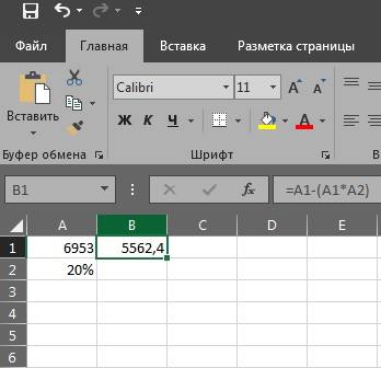
The fastest and by far the easiest way to display the sum in Excel is the AutoSum service. To use it, you must select the cells that contain the values you want to add, as well as the empty cell directly below them. In the "Formulas" tab, you must click on the "AutoSum" sign, after which the result of the addition appears in an empty cell.
The same method is available in reverse order. In an empty cell where you want to display the result of addition, you must put the cursor and click on the "AutoSum" sign. After clicking in the cell, a formula with a free summation range is formed. Use the cursor to select the range of cells whose values need to be added, and then press Enter.
Cells for addition can also be defined without selection by the cursor. The sum formula looks like: "=SUM(B2:B14)", where the first and last cells of the range are given in brackets. By changing the cell values in the Excel spreadsheet, you can adjust the summation range.
Sum of values to roll up
Excel allows you not only to sum up the values for some specific purposes, but also automatically counts the selected cells. Such information can be useful in cases where the task is not related to the summation of numbers, but consists in the need to look at the value of the sum at an intermediate stage. To do this without resorting to writing a formula, just select the desired cells and in the program command line at the very bottom, right-click on the word "Finish". In the context menu that opens, opposite the "Amount" column, the value of all cells will be displayed.
Simple addition formula in Excel
In cases where the values to be added are dispersed throughout the table, you can use a simple addition formula in an Excel spreadsheet. The formula has the following structure:
To create a formula in a free cell where the amount should be displayed, put an "equal" sign. Excel automatically reacts to this action as if it were a formula. Next, using the mouse, you need to select the cell with the first value, after which a plus sign is placed. Further, all other values are also entered into the formula through the addition sign. After the chain of values is typed, the Enter button is pressed. The use of this method is justified when adding a small number of numbers.
SUM Formula in Excel
Despite the almost automated process of using addition formulas in Excel, sometimes it’s easier on your own. In any case, their structure must be known in cases where the work is carried out in a document created by another person.
The SUM formula in Excel has the following structure:
SUM(A1;A7;C3)
When typing the formula yourself, it is important to remember that spaces are not allowed in the structure of the formula, and the sequence of characters must be clear.
Sign ";" is used to define a cell, in turn, the ":" sign sets the range of cells.
An important nuance is that when counting the values of the entire column, you do not need to set the range by scrolling to the end of the document, which has a border of over 1 million values. It is enough to enter a formula with the following values: =SUM(B:B), where the letters indicate the column to be calculated.
Excel also allows you to display the sum of all cells in a document without exception. To do this, the formula must be entered in a new tab. Let's assume that all the cells whose sums need to be calculated are located on Sheet1, in which case the formula should be written on Sheet2. The structure itself looks like this:
SUM(Sheet1!1:1048576), where the last value is the numeric value of the very last cell of Sheet1.
Hi all! This article will show you how to calculate the percentage of a number in Excel. For beginners who are just starting to learn Microsoft Office text programs, the Excel editor seems to be the most difficult. Almost endless tables, numerous functions and formulas, at first confuse even experienced PC users, but in fact, everything is much simpler than it might seem at first glance.
In this article, we will look at the basics and advantages of arithmetic work with excel using specific examples and tasks. In particular, we will get acquainted with the percentage increase formula, calculate percentages of total amounts, learn how to quickly and easily calculate percentage changes, and also learn many other percentage calculations that can be performed in Excel.
The skills of working with interest will certainly come in handy in various areas of life: find out the exact amount of tips in a cafe, bar or restaurant, calculate the income and expenses of an enterprise, calculate commission payments, deposit accruals, etc. Percentage calculations in Excel are more efficient and easier than on a calculator; take less time and can be organized into structured tables for reporting documentation or personal use.
The guide presented in the article will teach you the technique of quickly calculating interest without outside help. By learning some tricks, you will hone your skills and be able to productively carry out the percentage calculations you need, using the maximum capabilities of Excel.
Basic concepts of interest
The term "percent" (from English - percent) came into modern European terminology from the Latin language (per centum - literal "every hundred"). We all remember from the school curriculum that a percentage is a certain particle from a hundred parts of one whole. The mathematical calculation of interest is carried out by dividing: the fraction of the numerator is the desired part, and the denominator is an integer from which we calculate; Further, the result is multiplied by 100.
In the classic formula for calculating interest, this would look like this:
For example: the farmer collected 20 chicken eggs in the morning, of which he immediately put 5 to prepare breakfast. What percentage of the collected eggs was used for breakfast?
By doing simple calculations, we get:
| (5/20)*100 = 25% |
It is according to such an uncomplicated algorithm that we were all taught to use at school when we need to calculate percentages from any total amount. Calculation of interest in Microsoft Excel - takes place in many respects in a similar way, but in automatic mode. A minimum of additional intervention is required from the user.
Given the different conditions of potential tasks in the calculation, there are several types of formulas for calculating percentages in a particular case. Unfortunately, there is no universal formula for all occasions. Below, we will look at simulated problems with specific examples that will introduce you to the practice of using Excel to calculate percentages.
Basic formula for calculating interest in Excel
The basic formula for calculating interest is as follows:
If you compare this formula, which is used by Excel, with the formula that we considered above using the example of a simple problem, then you probably noticed that there is no operation with multiplication by 100. When calculating with percentages in Microsoft Excel, the user does not need to multiply the resulting division result per hundred, the program carries out this nuance automatically, if for the working cell, you previously set "Percentage Format".
And now, let's look at how the calculation of percentages in Excel makes it easier to work with data.
For example, let's imagine a grocery seller who writes a certain number of fruits ordered to him (Ordered) in the Excel column "B", and records the number of goods already delivered (Delivered) in column "C". To determine the percentage of completed orders, we will do the following:
- Write down the formula \u003d C2 / B2 into cell D2 and copy it down to the required number of lines;
- Next, click the command Percent Style (Percentage format) to get the display of the results of the arithmetic calculation as a percentage. The command button we need is located in the Home tab (Home) in the category of commands Number (Number)
- The result will immediately be displayed on the screen in column "D". We received information in percentage about the share of goods already delivered.
It is noteworthy that if you use any other program formula to sum up percentage calculations, the sequence of steps when calculating in Excel will still remain the same.
How to calculate percentage of a number in Excel without long columns
Or consider another simplified problem. Sometimes the user just needs to display a percentage of a whole number without additional calculations and structural divisions. The mathematical formula will be similar to the previous examples:
The task is as follows: find a number that is 20% of 400.
What should be done?
First stage
You need to assign a percentage format to the desired cell in order to immediately get the result in integers. There are several ways to do this:
- Enter the desired number with the "%" sign, then the program will automatically determine the desired format;
- By right-clicking on the cell, click "Cell Format" - "Percentage";
- Simply select a cell using the hot key combination CTRL+SHIFT+5;
Second phase
- Activate the cell in which we want to see the result of the count.
- In the line with the formula or immediately, directly in the cell, enter the combination = A2 * B2;
- In the cell of the column "C" we immediately get the finished result.
You can define percentages without using the "%" sign. To do this, you need to enter the standard formula =A2/100*B2. It will look like this:
This method of finding percentages from the amount also has the right to life and is often used in working with Excel.
Features of calculating percentage of the total amount in Excel
The above examples of calculating percentages are one of the few ways that Microsoft Excel uses. Now, we'll look at a few more examples of how percentages of the total can be calculated using different variations of the data set.
Example #1. The final calculation of the amount at the bottom of the table.
Quite often, when creating large tables with information, a separate “Total” cell is highlighted at the bottom, into which the program enters the results of summary calculations. But what if we need to calculate separately the share of each part in relation to the total number / amount? With such a task, the percentage calculation formula will look similar to the previous example with only one caveat - the reference to the cell in the denominator of the fraction will be absolute, that is, we use the "$" signs before the column name and before the line name.
Let's consider an illustrative example. If your current data is fixed in column B, and the total of their count is entered in cell B10, then use the following formula:
| =B2/$B$10 |
Thus, in cell B2, a relative reference is used so that it changes when we copy the formula to other cells in column B. It is worth remembering that the cell reference in the denominator must be left unchanged while copying the formula, which is why we will write it like $B$10.
There are several ways to create an absolute cell reference in the denominator: either you enter the $ symbol manually, or you select the required cell reference in the formula bar and press the F4 key on your keyboard.
In the screenshot, we see the results of calculating the percentage of the total. The data is displayed in percentage format with "tenths" and "hundredths" after the decimal point.
Example #2: Scatter parts of a sum on multiple lines
In this case, we imagine a table with numerical data, similar to the previous example, but only here, the information will be sorted into several rows of the table. This structure is often used in cases where you need to calculate the share of total profit / waste from orders for a particular product.
In this task, the SUMIF function will be used. This function will allow you to add only those values that meet specific, given criteria. In our example, the criterion will be the product we are interested in. When the results of the calculations are received, it will be possible to calculate the percentage of the total.
The "skeleton" of the formula for solving the problem will look like this:
Enter the formula in the same field as in the previous examples.
For even greater convenience of calculations, you can immediately enter the name of the product in the formula, well, or what you specifically need. It will look like this:
Using a similar algorithm, the user can obtain the counts of several products at once from one worklist. It is enough to summarize the results of the calculations for each of the positions, and then divide by the total amount. This is what the formula would look like for our fruit salesman if he wants to calculate percentage results for cherries and apples:
How percentage changes are calculated
The most popular and demanded task that is performed using the Excel program is calculating the dynamics of data changes in percentage terms.
Formula for calculating the increase / decrease in percentage of the amount
To quickly and conveniently calculate the percentage change between two values, A and B, use this formula:
| (B-A)/A = Percent change |
Using the algorithm when calculating real data, the user must clearly determine for himself where the value will be BUT, and where to put AT.
For example: Last year, the farmer harvested 80 tons of crops from the field, and this year the harvest was 100 tons. For the initial 100%, we take 80 tons of last year's harvest. Therefore, an increase in results by 20 tons means a 25% increase. But if that year, the farmer had a crop of 100 tons, and this year - 80, then the loss would be 20%, respectively.
To carry out more complex mathematical operations of a similar format, we adhere to the following scheme:
The purpose of this formula is to calculate the percentage fluctuations (fall and gain) in the cost of goods of interest in the current month (column C) in comparison with the previous one (column B). A lot of people represented small businesses, puzzle over numerous invoices, the dynamics of price changes, profits and expenses in order to reach the exact amount of the current cash flow. In fact, everything can be solved in just a couple of hours maximum, using the Excel function for calculating the comparative percentage dynamics.
Write the formula in the field of the first cell, copy it (the formula) into all the lines you need - drag the autofill marker, and also set the "Percentage Format" for cells with our formula. If everything is done correctly, you will get a table similar to the one shown below. Positive growth data is identified in black, while negative trends are indicated in red.
By analogy, you can enter the expense items of the family budget or a small business / store into the table and track the dynamics of profits and waste.
5 (100%) 10 votesMany novice users often wonder how to quickly calculate percentages in Excel or which formula is better to use in calculations.
Often this is necessary even for the simplest calculations, ranging from the household need to calculate a discount in a store to some accounting calculations, such as determining the amount to be paid for utilities.
Content:
Interest calculation
It is worth starting with the fact that the formula for calculating interest differs from the mathematical one we are familiar with. It looks like this:
Part/Whole = Percentage
An attentive user will immediately notice that there is not enough multiplication by 100 and this will be a correct remark. AT
from only in the program this is not necessary if you ask the cell "Percentage Format", the program will multiply on its own. Now let's look at all the necessary actions using an example.
Suppose we have a list of products (column A) and there is data on them - how many were pre-bought (column B), and how many of them were sold after (column C).
It is important for us to know what percentage of the purchased goods are sold (column D). To do this, we do the following:
- We enter the formula = C2 / B2 in cell D2, and in order not to do this with all rows, simply by selecting the autofill marker, copy it down as much as necessary.


Hello!
Many who do not use Excel - do not even imagine what opportunities this program gives! Just think: automatically add values from one formula to another, search for the desired lines in the text, add by condition, etc. - in general, in fact, a mini-programming language for solving "narrow" tasks (to be honest, for a long time I myself did not consider Excel as a program, and almost did not use it) ...
In this article I want to show a few examples of how you can quickly solve everyday office tasks: add something, subtract something, calculate the sum (including with a condition), substitute values from one table to another, etc. That is, this article will be something like a mini guide on learning the most necessary things for work (more precisely, to start using Excel and feel the full power of this product!).
It is possible that if you had read a similar article 15-17 years ago, I myself would have started using Excel much faster (and would have saved a lot of my time for solving "simple" (note: as I understand now) tasks)...
Note: All screenshots below are from Excel 2016 (as the newest to date).
Many novice users, after starting Excel, ask one strange question: "well, where is the table?". Meanwhile, all the cells that you see after starting the program are one big table!
Now to the main thing: in any cell there can be text, some number, or a formula. For example, the screenshot below shows one illustrative example:
- left: Cell (A1) contains the prime number "6". Note that when you select this cell, the formula bar (Fx) just shows the number "6".
- right : in cell (C1) it also looks like a simple number "6", but if you select this cell, you will see the formula "=3+3" - this is an important feature in Excel!

Just a number (on the left) and a calculated formula (on the right)
The bottom line is that Excel can count like a calculator if you select some cell, and then write a formula, for example "=3+5+8" (without quotes). You do not need to write the result - Excel will calculate it and display it in the cell (as in cell C1 in the example above)!
But you can write in formulas and add not just numbers, but also numbers already calculated in other cells. In the screenshot below, in cell A1 and B1, the numbers are 5 and 6, respectively. In cell D1, I want to get their sum - you can write the formula in two ways:
- first: "=5+6" (not very convenient, imagine that in cell A1 - we also have a number calculated according to some other formula and it changes. You won’t substitute a number instead of 5 every time?!);
- the second: "=A1+B1" - and this perfect option, just add the value of cells A1 and B1 (regardless of what numbers are in them!)

Add cells that already have numbers
Extending a formula to other cells
In the example above, we added two numbers in column A and B in the first row. But then we have 6 lines, and most often in real problems you need to add numbers in each line! To do this, you can:
- on line 2 write the formula "=A2+B2" , on line 3 - "=A3+B3", etc. (this is long and tedious, this option is never used);
- select cell D1 (which already has a formula), then move the mouse pointer to the right corner of the cell so that a black cross appears (see screenshot below). Then hold down the left button and stretch the formula to the entire column. Convenient and fast! (Note: You can also use Ctrl+C and Ctrl+V combinations for formulas (copy and paste respectively)).

By the way, pay attention to the fact that Excel itself has substituted formulas in each line. That is, if you now select a cell, say D2, you will see the formula "=A2+B2" (i.e. Excel automatically fills in the formulas and returns the result immediately) .
How to set a constant (a cell that will not change when copying a formula)
Quite often it is required in formulas (when you copy them) that some value does not change. Let's say a simple task: convert prices in dollars into rubles. The cost of the ruble is set in one cell, in my example below it is G2.
Next, in cell E2, the formula "=D2*G2" is written and we get the result. Only now, if we stretch the formula, as we did before, we will not see the result in other lines, because Excel in line 3 will put the formula "D3*G3", in the 4th line: "D4*G4", etc. G2 must remain G2 everywhere...
To do this - just change cell E2 - the formula will look like "=D2*$G$2". Those. dollar sign $ - allows you to set a cell that will not change when you copy the formula (i.e. get a constant, example below)...

How to calculate the sum (SUM and SUMIFS formulas)
You can, of course, write formulas manually by typing "=A1+B1+C1" and so on. But Excel has faster and more convenient tools.
One of the easiest ways to add up all selected cells is to use the option autosums (Excel will write the formula itself and paste it into the cell).
- first select the cells (see screenshot below);
- then open the section "Formulas";
- The next step is to press the "Autosum" button. Under the cells you selected, the result of the addition will appear;
- if you select the cell with the result (in my case, this is the cell E8) - then you will see the formula "=SUM(E2:E7)" .
- thus writing the formula "=SUM(xx)", where instead of xx put (or select) any cells, you can read a wide variety of ranges of cells, columns, rows...

Quite often, when working, it is required not just the sum of the entire column, but the sum of certain rows (i.e. selectively). Suppose a simple task: you need to get the amount of profit from some worker (exaggerated, of course, but the example is more than real).
I will use only 7 rows in my table (for clarity), the real table can be much larger. Suppose we need to calculate all the profit that "Sasha" made. What the formula will look like:
- "=SUMIFS(F2:F7 ;A2:A7 ;"Sasha") " - (note: pay attention to the quotation marks for the condition - they should be like in the screenshot below, and not as it is written on my blog now). Also note that Excel, when driving in the beginning of a formula (for example, "SUM ..."), itself prompts and substitutes possible options - and there are hundreds of formulas in Excel!;
- F2:F7 - this is the range over which the numbers from the cells will be added (summed up);
- A2:A7 is the column by which our condition will be checked;
- "Sasha" is a condition, those lines in which "Sasha" will be in column A will be added (pay attention to the indicative screenshot below).

Note: there can be several conditions and you can check them in different columns.
How to count the number of rows (with one, two or more conditions)
Quite a typical task: to calculate not the sum in the cells, but the number of rows that satisfy some condition. Well, for example, how many times the name "Sasha" occurs in the table below (see screenshot). Obviously, 2 times (but this is because the table is too small and taken as a good example). How can this be calculated as a formula? Formula:
"=COUNTIF(A2:A7 ,A2 )" - where:
- A2:A7- the range in which lines will be checked and counted;
- A2- a condition is set (note that you could write a condition like "Sasha", or you can just specify a cell).
The result is shown on the right side of the screenshot below.

Now imagine a more extended task: you need to count the lines where the name "Sasha" occurs, and where in the AND column there will be the number "6". Looking ahead, I will say that there is only one such line (screen with an example below).
The formula will look like:
=COUNTIFS(A2:A7 ;A2 ;B2:B7 ;"6") (note: pay attention to the quotes - they should be like in the screenshot below, and not like mine), where:
A2:A7 ;A2- the first range and search condition (similar to the example above);
B2:B7 ;"6"- the second range and the search condition (note that the condition can be specified in different ways: either specify a cell, or simply write text/number in quotes).

How to calculate the percentage of the amount
It's a very common question that I often come across. In general, as far as I can imagine, it occurs most often - due to the fact that people get confused and do not know what percentage is looking for (and in general, they do not understand the topic of interest well (although I myself am not a great mathematician, and yet ...)).
The simplest way, in which it is simply impossible to get confused, is to use the "square" rule, or proportion. The whole essence is shown on the screen below: if you have a total amount, let's say in my example this number is 3060 - cell F8 (i.e. this is 100% profit, and "Sasha" made some part of it, you need to find which ... ).
In proportion, the formula will look like this: =F10*G8/F8(i.e. cross by cross: first we multiply two known numbers diagonally, and then divide by the remaining third number). In principle, using this rule, it is almost impossible to get lost in percentages.

Actually, this concludes this article. I'm not afraid to say that having mastered everything that is written above (and only "heels" of formulas are given here) - you will be able to learn Excel on your own, flip through help, watch, experiment, and analyze. I will say even more, everything that I described above will cover many tasks, and will allow you to solve the most common ones that you often puzzle over (if you don’t know the capabilities of Excel), and you don’t know how to do it faster ...