Microsoft Excel- this is a program that is needed, first of all, by accountants and economists. After all, in it you can compile tables (reports), make calculations of any complexity, draw up diagrams. Moreover, all this can be done without much difficulty and incredible knowledge.
Microsoft Excel is a large table into which you can enter data, that is, print words and numbers. Also, using the functions of this program, you can perform various manipulations with numbers (add, subtract, multiply, divide and much more).
Many people think that Microsoft Excel is just tables. That is, they are convinced that all tables on a computer are compiled only in this program. This is not entirely true.
Yes, indeed, Microsoft Excel is a spreadsheet. But this program is needed, first of all, for calculations. If you need not only to draw a table with words and numbers, but also to perform any actions with the numbers (add, multiply, calculate the percentage, etc.), then you need to use Microsoft program Excel.
Comparing Microsoft Excel with Microsoft Word then Microsoft Excel is of course more complicated. And it is better to start working in this program after you have mastered Word. It will take a long time to learn Microsoft Excel thoroughly.
When working with Microsoft Excel, use keyboard shortcuts instead of the mouse. Using keyboard shortcuts, you can open, close documents and sheets, move through the document, execute various actions over cells, perform calculations, etc. Using keyboard shortcuts will make it easier and faster to work with the program.
Keyboard shortcuts quick call using the CTRL key:
CTRL + PgUp Switch between sheet tabs from left to right.
CTRL + PgDn Switch between sheet tabs from right to left.
CTRL + SHIFT + (Show hidden lines in the selection.
CTRL + SHIFT + & Paste outer borders into selected cells.
CTRL + SHIFT + _ Remove outer borders from selected cells.
CTRL + SHIFT + ~ Apply Shared number format.
CTRL + SHIFT + $ Apply currency format with two decimal places (negative numbers appear in parentheses).
CTRL + SHIFT +% Apply percentage format without fractional part.
CTRL + SHIFT + ^ Apply exponential number format with two decimal places.
CTRL + SHIFT + # Apply date format with day, month and year.
[email protected] Apply time format with hour and minute display and AM or PM indices.
CTRL + SHIFT +! Apply a number format with two decimal places, a thousands separator and a minus sign (-) for negative values.
CTRL + SHIFT + * Select the current area around the active cell (data area bounded by empty rows and empty columns).
CTRL + SHIFT + "Copy the contents of the top cell to the current cell or formula bar.
CTRL + SHIFT + plus sign (+) Display the Add Cells dialog box for inserting blank cells.
CTRL + Minus Sign (-) Display the Delete Cells dialog box to delete the selected cells.
CTRL +; Insert the current date.
CTRL + `Switch between displaying cell values and formulas in the worksheet.
CTRL + ’Copy the formula in the top cell to the current cell or to the formula bar.
CTRL + 1 Display the Format Cells dialog box.
CTRL + 2 Apply or remove boldface.
CTRL + 3 Apply or remove italics.
CTRL + 4 Apply or remove underline.
CTRL + 5 Strikethrough text or remove strikethrough.
CTRL + 6 Toggle between hiding and showing objects.
CTRL + 8 Show or hide outline symbols.
CTRL + 9 Hide selected lines.
CTRL + 0 Hide selected columns.
CTRL + A Select the entire sheet.
If the sheet contains data, CTRL + A selects the current region. Pressing CTRL + A again selects the entire sheet.
CTRL + B Apply or remove bold.
CTRL + C Copy selected cells.
CTRL + D Uses the Fill Down command to copy the content and format the top cell of the selection to all the bottom cells.
CTRL + F Displays the Find and Replace dialog box with the Find tab selected.
SHIFT + F5 also brings up this tab, while SHIFT + F4 repeats last action on the Find tab.
The keyboard shortcut CTRL + SHIFT + F displays the Format Cells dialog box with the Font tab selected.
CTRL + G Displays the Transition dialog box.
The F5 key also displays this dialog box.
CTRL + H Displays the Find and Replace dialog box with the Replace tab selected.
CTRL + I Apply or remove italics.
CTRL + K Displays the Insert Hyperlink dialog box for new hyperlinks or Edit Hyperlink for an existing selected hyperlink.
CTRL + L Displays the Create Table dialog box.
CTRL + N Creates a new blank workbook
CTRL + O Displays the Open Document dialog box for opening or searching for a file.
The keyboard shortcut CTRL + SHIFT + O selects all cells that contain comments.
CTRL + P Displays the Print tab in view Microsoft Office Backstage, Microsoft Representation Office Backstage.
The keyboard shortcut CTRL + SHIFT + P displays the Format Cells dialog box with the Font tab selected.
CTRL + R Uses the Fill Right command to copy the content and format the left-most cell of the selected area to all cells to the right.
CTRL + S Saves the work file with the current file name in the current location and in the existing format.
CTRL + T Displays the Create Table dialog box.
CTRL + U Apply or remove underline.
CTRL + SHIFT + U expands and collapses the formula bar.
CTRL + V Pastes the contents of the clipboard at the insertion point and replaces the selection. Functions only when there is an object, text, or cell content on the clipboard.
Pressing CTRL + ALT + V opens a dialog box Paste special... It is available only after copying or cutting an object, text, or cell content on a sheet or in another program.
CTRL + W Closes the selected book window.
CTRL + X Deletes the contents of the selected cells.
CTRL + Y Repeats the last command or action, if possible.
CTRL + Z Uses the Undo command to undo the last command or delete the last entry entered.
F1
Displaying the task pane Microsoft Help Excel.
The keyboard shortcut CTRL + F1 shows or hides the ribbon.
The keyboard shortcut ALT + F1 creates a chart with data in the current area.
The keyboard shortcut ALT + SHIFT + F1 adds a new sheet to the workbook.
F2
Opens active cell for editing and places the cursor at the end of the cell content. Also moves the insertion point to the formula bar if editing mode in a cell is off.
The SHIFT + F2 keyboard shortcut adds or modifies cell comments.
The shortcut keys CTRL + F2 displays the region preview Print on the Print tab in Backstage view Backstage view.
F3
Displays the Insert Name dialog box. Available only if available in workbook created names.
SHIFT + F3 displays the Insert Function dialog box.
F4
Repeats the last command or action, if possible.
When a cell or range reference is selected in a formula, the F4 key toggles between all possible absolute and relative values.
The keyboard shortcut CTRL + F4 closes the selected book window.
The keyboard shortcut ALT + F4 closes Microsoft Excel.
F5
Displays the Transition dialog box.
The keyboard shortcut CTRL + F5 restores the size of the selected workbook window.
F6
Switches the insertion point between sheet, ribbon, task pane, and zoom controls. In split sheets (View menu, Window group, Freeze Areas section, Split Window command), when you switch between panels and the ribbon area using the F6 key, the split areas are also included.
The SHIFT + F6 keyboard shortcut switches control between the sheet, zoom controls, task pane, and ribbon.
If more than one book is open, the CTRL + F6 keyboard shortcut switches the insertion point to the next book window.
F7
Displays the Spelling dialog box for spellchecking in the active sheet or selection.
If the book window is not maximized, the keyboard shortcut CTRL + F7 executes the Move command. Use the arrow keys to move the window and press ENTER or ESC to cancel.
F8
Switch to selection mode and exit from it. When enabled, the status bar displays Expand Selection, and the arrow keys expand selection.
The SHIFT + F8 keyboard shortcut lets you use the arrows to add non-adjacent cells or a range to a selection.
CTRL + F8 executes the Size command (on the Book Window Control menu) if the window is not maximized.
The keyboard shortcut ALT + F8 displays the Macro dialog box, which allows you to create, run, modify, and delete macros.
F9
Calculates all sheets of all open workbooks.
SHIFT + F9 calculates the active sheet.
CTRL + ALT + F9 calculates all sheets of all open workbooks, regardless of whether they have changed since the last calculation.
CTRL + ALT + SHIFT + F9 validates dependent formulas and then recalculates cells in all open books, including cells not marked for calculation.
The shortcut keys CTRL + F9 minimizes the book window to an icon.
F10
Turns tooltips on and off (the same happens when you press the ALT key).
The keyboard shortcut SHIFT + F10 displays context menu for the selected item.
The keyboard shortcut ALT + SHIFT + F10 displays the error check button menus or messages.
The shortcut keys CTRL + F10 expand or restore original size selected book window.
F11
Creates a chart with data from the current range on a separate sheet.
The keyboard shortcut SHIFT + F11 inserts a new sheet into the workbook.
The shortcut keys ALT + F11 opens the editor Microsoft Visual Basic for Applications in which you can create a VBA macro.
With the release of Excel 2010, Microsoft has almost doubled the functionality of the program, adding many improvements and innovations, many of which are not immediately noticeable. Whether you're an experienced user or a newbie, there are many ways to make your Excel experience easier. We will tell you about some of them today.
Select all cells with one click
All cells can be selected with a combination Ctrl keys+ A, which, by the way, works in all other programs. However, there is an easier way to highlight. By clicking on the button in the corner Excel worksheet, you will select all cells with one click.
Opening multiple files at the same time

Instead of opening each one Excel file individually, they can be opened together. To do this, highlight the files you want to open and press Enter.
Navigating Excel files
When you have multiple workbooks open in Excel, you can easily navigate between them using the Ctrl + Tab key combination. This feature is also available throughout Windows system and it can be used in many applications. For example, to switch tabs in the browser.
Adding New Buttons to the Quick Access Toolbar

Standard in the panel quick access Excel there are 3 buttons. You can change this amount and add the ones that you need exactly.
Go to the menu "File" ⇒ "Options" ⇒ "Quick Access Toolbar". Now you can select whatever buttons you want.
Diagonal line in cells

Sometimes there are situations when you need to add a diagonal line to the table. For example, to separate date and time. To do this, on the main Excel page click on the familiar border icon and select "Other Borders".
Add empty rows or columns to a table
Inserting a single row or column is straightforward. But what if you need to insert many more? Select the required number of rows or columns and click "Insert". After that, select the place where you want to move the cells, and you will get the required amount blank lines.
High-speed copying and movement of information

If you need to move any information (cell, row, column) in Excel, select it and move the mouse over the border to change the pointer. After that, move the information to the place that you need. If you need to copy information, do the same, but holding down the Ctrl key.
Quickly remove blank cells

Empty cells are the bane of Excel. Sometimes they just appear out of nowhere. To get rid of them all in one go, select the column you want, go to the Data tab and click Filter. A downward arrow appears above each column. Clicking on it will take you to a menu that will help you get rid of empty fields.
Advanced Search
Pressing Ctrl + F, we get to the search menu, with which you can search for any data in Excel. However, its functionality can be extended by using the "?" and "*". The question mark is responsible for one unknown symbol, and the asterisk - for several. They are worth using if you are not sure what the search query looks like.
If you need to find a question mark or an asterisk and you do not want Excel to search for an unknown character instead, then put "~" in front of them.
Copying unique records

Unique records can be useful when you need to highlight non-repeating information in a table. For example, one person of each age. To do this, select the required column and click "Advanced" to the left of the "Filter" item. Select the source range (where to copy from) and the range where you want to place the result. Don't forget to check the box.
Sample creation

If you are doing a survey in which only males between 19 and 60 can participate, you can easily create a similar sample with using Excel... Go to the menu item "Data" ⇒ "Data check" and select required range or some other condition. By entering information that does not meet this condition, users will receive a message that the information is incorrect.
Fast navigation with Ctrl and arrow keys
Pressing Ctrl + arrow, you can move to the extreme points of the sheet. For example, Ctrl + ⇓ will move the cursor to lower part sheet.
Transpose information from a column to a row

Enough useful function, which is not needed very often. But if you suddenly need it, you are unlikely to transpose one by one. There is a special paste for transposition in Excel.
Copy the range of cells to be transposed. Then click right click on Right place and select paste special.
How to hide information in Excel

I don’t know why this might be useful, but nevertheless there is such a function in Excel. Select the desired range of cells, click Format ⇒ Hide or Show and select the desired action.
Combining text with "&"

If you need to combine text from several cells into one, you do not need to use complex formulas. It is enough to select the cell in which the text will be connected, press "=" and sequentially select the cells, putting "&" in front of each.
Changing the case of letters
Using certain formulas, you can change the case of the entire text information in Excel. The UPPERCASE function capitalizes all letters and LOWCASE makes all letters lowercase. PROPNACH capitalizes only the first letter of each word.
Entering information with zeros at the beginning
If you enter in Excel number 000356, the program will automatically convert it to 356. If you want to leave zeros at the beginning, precede the number with an apostrophe "’ ".
Speeding up difficult words

If you often enter the same words, you will be delighted to know that Excel has AutoCorrect. It is very similar to AutoCorrect in smartphones, so you will immediately understand how to use it. It can be used to replace repetitive designs with abbreviations. For example, Ekaterina Petrova - EP.
More information

In the lower right corner you can follow various information... However, few people know that by right-clicking there, you can remove unnecessary lines and add the necessary lines.
Rename a sheet with a double click
This is the easiest way to rename a sheet. Just double-click on it with the left mouse button and enter a new name.
How often do you use Excel? If yes, then you probably have your own secrets of working with this program. Share them in the comments.
Thank you for your interest in our site. The IT company has existed since 2006 and provides IT outsourcing services. Outsourcing is the transfer of necessary, but non-core work for the company to another organization. In our case, these are: creation, support and maintenance of sites, promotion of sites in search engines, support and administration of servers under Debian management GNU / Linux.
Joomla Websites
In the current age of information, the site is de facto becoming at least business card organization, and often one of the business tools. Already, sites are being created not only for organizations and individuals, but also for individual goods, services and even events. Today, the site is not only a source of advertising for a giant audience, but also a tool for sales and making new contacts. We create websites using CMS Joomla! This site management system is simple and intuitive. It is very widespread and, therefore, the Internet contains about it a large number of information. Finding a Joomla specialist is also easy. And you don't have to go far! Our company IT specialist is engaged in the maintenance and support of sites on Joomla! We'll take it all engineering works, we will take care of all the correspondence with the hoster and the domain registrar, fill the site and update the information on it. And while Joomla is easy to manage, it's intuitive. But will you yourself regularly perform necessary work on the site? How long will they take from you? If you want to concentrate on your business, then entrust the support of your site to us. We will do our best to make the site live and benefit its owner.
If you are a commercial organization that advertises or sells its goods and services on the Internet, then you just need to promote your site in search engines. After all, in order to sell something you have to, at least, to see it, to know about it. And we will help you with this, we will promote your Joomla site in the search engines. Depending on the competition and the budget allocated for the promotion, your site will occupy a worthy position in search results... The site will increase your profits!
Debian servers
Sooner or later, striving for openness and transparency of their business, many companies are faced with the need to ensure the license purity of the software... However, the costs of licensing fees are not always acceptable, especially for small and medium-sized businesses. The way out of this difficult situation is the decision to switch to Open source technologies. One of the areas of Open Source is the operating Linux system(Linux). Our employees are specialized in Debian Linux(Debian Linux). It is the oldest and most stable distribution operating system Linux. We offer you services for the implementation of Debian Linux in your enterprise, configuration, maintenance and support of servers.
Information and advertising
Excel is not the friendliest program in the world. Regular user uses only 5% of its capabilities and has a poor idea of what treasures are hidden by its bowels. H&F read the advice of Excel-guru and learned how to compare price lists, hide classified information from prying eyes and compose analytical reports in a couple of clicks. (Oh "kay, sometimes there are 15 clicks.)
Import of exchange rates


In Excel, you can set up a constantly updated exchange rate.
Select the Data tab from the menu.
Click on the "From the Web" button.
In the window that appears, in the "Address" line, enter http://www.cbr.ru and press Enter.
When the page is loaded, black and yellow arrows will appear on the tables that Excel can import. Clicking on such an arrow marks the table for import (picture 1).
Mark the table with the exchange rate and click the "Import" button.
The course will appear in the cells on your worksheet.
Right-click on any of these cells and select the Range Properties command from the menu (Figure 2).
In the window that appears, select the update rate for the course and click "OK".
Super secret leaf


Let's say you want to hide some of the sheets in Excel from other users working on the workbook. If you do this in the classic way- right-click on the sheet tab and click on "Hide" (picture 1), then the name hidden leaf will still be visible to another person. To make it completely invisible, you need to act like this:
Press ALT + F11.
On the left you will see an elongated window (picture 2).
At the top of the window, select the sheet number you want to hide.
- At the bottom, at the very end of the list, find the "Visible" property and make it "xlSheetVeryHidden" (Figure 3). Now no one but you will know about this sheet.
No retroactive changes


Before us is a table (picture 1) with empty fields "Date" and "Quantity". Vasya's manager will indicate today how many carrots he sold per day. How do you prevent him from retroactively making changes to this table in the future?
Place the cursor on the cell with the date and select the "Data" item from the menu.
Click on the "Data Check" button. A table will appear.
In the drop-down list "Data type" select "Other".
In the column "Formula" we write = A2 = TODAY ().
Uncheck the box "Ignore empty cells"(Picture 2).
Click the "OK" button. Now, if a person wants to enter a different date, a warning message will appear (picture 3).
You can also prohibit changing the numbers in the "Amount" column. We put the cursor on the cell with the quantity and repeat the algorithm of actions.
Prohibiting the entry of duplicates


You want to enter a list of products in the price list so that they do not repeat. You can prohibit this repeat. The example shows the formula for a column of 10 cells, but of course there can be any number of them.
Select cells A1: A10, which will be subject to the ban.
In the "Data" tab, click the "Data Check" button.
In the "Parameters" tab from the "Data type" drop-down list, select the "Other" option (picture 1).
In the "Formula" column we drive in = COUNTIF ($ A $ 1: $ A $ 10; A1)<=1.
In the same window, go to the "Error message" tab and enter the text that will appear when you try to enter duplicates (picture 2).
Click "OK".
Selective summation

Here is a table from which you can see that different customers several times bought different goods from you for certain amounts. You want to know how much a customer named ANTON bought Boston Crab Meat from you.
In cell G4, you enter the customer's name ANTON.
Cell G5 contains the name of the Boston Crab Meat product.
You stand on cell G7, where the amount will be calculated, and write the formula for it (= SUM ((C3: C21 = G4) * (B3: B21 = G5) * D3: D21)). At first, it scares you with its volume, but if you write gradually, then its meaning becomes clear.
First, enter (= SUM and open parentheses that contain three factors.
The first multiplier (C3: C21 = G4) looks for references to ANTON in the specified list of clients.
The second multiplier (B3: B21 = G5) does the same with Boston Crab Meat.
The third factor D3: D21 is responsible for the cost column, after which we close the parentheses.
Pivot table


You have a table (picture 1), which indicates which product, to which customer, for what amount a particular manager sold. When it grows, it is very difficult to select individual data from it. For example, you want to understand how much carrots were sold for or which of the managers completed the most orders. Pivot tables are available in Excel to solve these problems. To create it, you need:
In the "Insert" tab, click the "Pivot Table" button.
In the window that appears, click "OK" (picture 2).
A window will appear in which you can create a new table using only the data you are interested in (picture 3).
Sales receipt


To calculate the total order amount, you can proceed as usual: add a column in which you need to multiply the price and quantity, and then calculate the amount for this column (picture 1). If you stop being afraid of formulas, you can do it more gracefully.
Select cell C7.
Enter = SUM (.
Select the range B2: B5.
We enter an asterisk, which in Excel is a multiplication sign.
Select the range C2: C5 and close the bracket (picture 2).
Instead of Enter, when writing formulas in Excel, you need to enter Ctrl + Shift + Enter.
Price comparison


This example is for advanced Excel users. Let's say you have two prices and you want to compare their prices. On the 1st and 2nd pictures we have prices from May 4 and 11, 2010. Some of the goods in them do not match - here's how to find out what kind of goods they are.
Create another sheet in the book and copy the lists of goods from both the first and the second price lists into it (picture 3).
To get rid of duplicate products, select the entire list of products, including its name.
In the menu, select "Data" - "Filter" - "Advanced filter" (picture 4).
In the window that appears, mark three things: a) copy the result to another location; b) put the result in the range - select the place where you want to write the result, in the example this is cell D4; c) put a tick on "Unique records only" (picture 5).
Press the "OK" button and, starting from cell D4, we get a list without duplicates (picture 6).
We delete the original list of goods.
We enter the formula = D5-C5 in the comparison column, which will calculate the difference (picture 7).
It remains to automatically load the values from the prices into the columns "May 4" and "May 11". To do this, use the function: = VLOOKUP (desired_value; table; column_number; interval_view).
- "Lookup_value" is the line that we will look for in the price table. The easiest way is to search for products by their name (picture 8).
- "Table" is an array of data in which we will search for the value we need. It must refer to the table containing the price list from the 4th (picture 9).
- "Column_number" is the ordinal number of the column in the range that we set to search for data. For the search, we have defined a two-column table. The price is contained in the second of them (picture 10).
Interval_view. If the table in which you are looking for a value is sorted in ascending or descending order, you must set the value TRUE, if not sorted, write FALSE.
Stretch the formula down, remembering to anchor the ranges. To do this, place a dollar sign in front of the column letter and in front of the line number (this can be done by highlighting the desired range and pressing the F4 key).
The final column reflects the difference in prices for those items that are in both prices. If # N / A is displayed in the final column, it means that the specified product is only in one of the prices, and therefore, the difference cannot be calculated.
Investment appraisal


In Excel, you can calculate the net present value (NPV), that is, the sum of the discounted values of the flow of payments to date. In the example, the NPV is calculated based on one investment period and four income generation periods (line 3 “Cash flow”).
The formula in cell B6 calculates NPV using a financial function: = NPV ($ B $ 4; $ C $ 3: $ E $ 3) + B3 (Figure 1).
In the fifth line, the calculation of the discounted flow in each period is found using two different formulas.
In cell C5, the result is obtained thanks to the formula = C3 / ((1 + $ B $ 4) ^ C2) (picture 2).
In cell C6, the same result is obtained through the formula (= SUM (B3: E3 / ((1 + $ B $ 4) ^ B2: E2))) (picture 3).
Comparison of investment proposals
In Excel, you can compare which of the two investment offers is more profitable. To do this, you need to write out in two columns the required volume of investments and the amount of their phased return, and also separately indicate the discount rate of investment in percent. Using this data, you can calculate the net present value (NPV).
In a free cell, you need to enter the formula = npv (b3 / 12, A8: A12) + A7, where b3 is the discount rate, 12 is the number of months in a year, A8: A12 is a column with numbers for a phased return on investment, A7 is the required amount of investments.
The net present value of another investment project is calculated using exactly the same formula.
Now they can be compared: whoever has more NPV, that project is more profitable.
ANTHONY DOMANICO. 11 tricks for Excel power users. PCWorld.
Knowing these features - from PivotTables to Power View - will help you join the ranks of the spreadsheet professional.
Microsoft Excel users are divided into two categories: the first one can barely cope with small tables, the second one amazes colleagues with complex charts, powerful data analysis and the magic of effective use of formulas and macros. The eleven tricks that we will look at in this article will help you become a full member of the second group.
VLOOKUP helps you collect data scattered on different sheets or stored in different Excel workbooks and put it in one place for reporting and calculating totals.
Suppose you are dealing with items sold in a retail store. Each item is usually assigned a unique inventory number that can be used as a link to the VLOOKUP. The formula "VLOOKUP" looks for the corresponding identifier on another sheet and substitutes from there the description of the product, its price, stock level and other data into the specified place in the workbook.
.jpg)
The VLOOKUP function helps you find information in large tables containing, for example, a list of available assortments.
Insert the "VLOOKUP" function into the formula, specifying in its first argument the desired value by which the link is made (1). In the second argument, specify the range of cells in which to select (2), in the third, the number of the column from which the data will be substituted, and in the fourth, enter the value FALSE if you want to find an exact match, or TRUE if you need the closest approximate variant ( 4).
Creating charts
To create a chart, enter data in Excel with the column headings (1), select the "Charts" item (2) on the "Insert" tab and specify the required chart type. Excel 2013 has a Recommended Charts tab (3) with types that match the data you entered. After defining the general nature of the chart, Excel opens the "Design" tab, where you can make more precise adjustments to it. The huge number of parameters present here allows you to give the diagram the appearance that you need.
.jpg)
In Excel 2013, there is a Recommended Charts tab that displays chart types that match the data you entered.
Functions "IF" and "ESLIOSHIBKA"
IF and IFERROR are some of the most popular Excel functions. The IF function allows you to define a conditional formula that, when a condition is met, calculates one value, and when it is not met, another. For example, students who received 80 points or more for the exam (the grades are in column C) can be assigned the sign "Pass", and those who received 79 points or less - the sign "Failed".
The IFERROR function is a special case of the more general IF function. It returns some specific value (or empty value) if an error occurs during the calculation of the formula. For example, when the VLOOKUP function is executed over another sheet or table, the IFERROR function may return an empty value in cases where VLOOKUP does not find the desired parameter specified by the first argument.
.jpg)
The IF function calculates the result based on the condition you specify.
Pivot table
A PivotTable is essentially a summary table that allows you to count the cardinality and calculate the average, sum, and other functions based on user-defined pivot points. Excel 2013 adds Featured Pivot Tables to make it easier to create tables that display the data you want.
For example, to calculate the average score of students based on their age, move the "Age" field to the Rows section (1), and the graded fields to the "Values" section (2). In the value menu, select the "Value field parameters" item and specify "Average" as the operation (3). In the same way, you can calculate the results for other categories, for example, calculate the number of those who passed and did not pass the exam depending on gender.
.jpg)
The pivot table is a tool for performing various final calculations over the table in accordance with the selected control points.
Pivot chart
Pivot charts have the characteristics of both pivot tables and traditional Excel charts. A pivot chart allows you to quickly and easily create an easy-to-understand visual representation of complex datasets. Pivot charts support many of the features of traditional charts, including series, categories, and more. The ability to add interactive filters allows you to manipulate selected subsets of the data.
Excel 2013 introduces Recommended Pivot Charts. Click the Insert tab, go to the Charts section and select Recommended Charts. Move your mouse over your selection to see how it will look. To manually create a PivotChart, click the PivotChart button on the Insert tab.
.jpg)
Pivot charts help you get an easy-to-read view of complex data.
Instant fill
Perhaps the best new feature in Excel 2013 - "Flash Fill" - allows you to effectively solve everyday tasks associated with the rapid transfer of the necessary blocks of information from adjacent cells. In the past, when working with a column in the Last Name, First Name format, the user had to manually extract the names from the column or find some very complex workarounds.
Suppose now that the same column of last names and first names is present in Excel 2013. You just need to enter the first person's first name in the cell (1) nearest to the right and select Fill and Instant Fill on the Home tab. Excel will automatically extract all other names and fill them in the cells to the right of the original ones.
.jpg)
"Flash Fill" allows you to extract the necessary blocks of information and fill in adjacent cells.
Fast analysis
The new Excel 2013 Quick Analysis tool helps you create charts faster from simple datasets. After the data is selected, a characteristic icon (1) appears next to the lower right corner of the selected area. By clicking on it, you go to the "Quick analysis" menu (2).
The menu contains tools for Formatting, Charts, Totals, Tables, and Sparklines. By clicking on these tools, you can see the capabilities they support.
.jpg)
Fast analysis speeds up work with simple datasets.
Power View
Power View, an interactive data exploration and visualization tool, is designed to extract and analyze large amounts of data from external sources. In Excel 2013, to invoke the Power View function, click the Insert tab (1) and click the Reports button (2).
Reports created with Power View are already presentation-ready and support Reading and Full Screen View modes. An interactive version of them can even be exported to PowerPoint. The business intelligence guides on the Microsoft website will help you become an expert in this area in no time.
.jpg)
Power View allows you to create interactive, presentation-ready reports.
Conditional formatting
Excel's advanced conditional formatting features make it easy and quick to highlight the data you want. The corresponding control is located on the Home tab. Select the range of cells you want to format and click the Conditional Formatting button (2). The submenu "Cell selection rules" (3) lists the most common formatting conditions.
.jpg)
Conditional formatting allows you to highlight the desired areas of data with minimal effort.
Transpose columns to rows and vice versa
Sometimes there is a need to swap rows and columns in a table. To do this, copy the required area to the clipboard, right-click on the upper left cell of the area into which you are pasting and select "Paste Special" from the context menu. In the window that appears on the screen, check the box "Transpose" and click OK. Excel will do the rest for you.
.jpg)
The Paste Special feature allows you to transpose columns and rows.
The most important keyboard shortcuts
The keyboard shortcuts shown here are especially useful for quickly navigating Excel spreadsheets and performing common operations.
.jpg)