Graph in Word will help to visually show numerical data.Here we will consider three optionshow to make a graph in Word.
First option.
How to make a graph in Word.
We put the cursor in the place of the page where we will place the chart. In the "Illustrations" section, click on the "Diagram" function. In the window that appears, select the "Chart" section and select the type of chart.
The "Templates" section of the window will contain templates for our charts, which we will save as a template.Click "OK". We have opened an Excel workbook in a new window with approximate data, because the graph is built on data from the Excel table.
And a graph appeared on the Word page.

Now we need to enter our data into this Excel table and automatically a graph in Word will be built on this data. To add rows, columns in an Excel table for a graph, you need to drag the lower right corner of the Excel table. This method inserts the chart, but does not update it if the data in the table changes. We use it when it is not necessary for the data to change.

After the graph was drawn, new bookmarks appeared in Word - "Working with charts".
"Constructor" tab Chart Tools tabs- in the "Type" section, you can change the type of schedule, save the schedule as a template for future work.
In the "Data" section, you can swap the rows and columns in the chart, change the data.
In the "Chart layouts" section, you can change the appearance of the chart, for example - to a chart with a title, with additional lines, data areas.
In the "Chart Styles" section, you can choose the appearance of the chart - color, bold lines, etc.
Layout tab.
Section "Current Fragment" - here you can customize any part of the chart by selecting it from the list. For example, let's choose - "Legend". This area is highlighted with a frame on the chart.

Function "Format of selected fragment" - you can click on any fragment of the chart, click on this function and a dialog box will come out. There are a lot of things you can change here.
Here the whole area of ​​the graph, chart is selected, and the dialog box is called "Format Chart Area".If we select the area of ​​the chart itself (colored lines of the chart), then the dialog box will be called "Plotting area format". In general, you can select any part of the chart and customize it.
"Insert" button - you can insert a picture, shape, inscription into the chart.
Section "Signatures" - you can remove or move different signatures in the chart field - names, data, etc.
Data Table button - you can place a data table (not Excel).
"Format" tab - here you can select the style of the shape, any section of the chart, the color and font of the labels, change the size of the chart, charts, adjust the position of the chart on the page, for example, so that the text flows around the chart or not, etc. How to work with inserted images, read the article "How to insert a photo, picture into a Word document".Here we have added data to an Excel spreadsheet and made a lot of changes in the graph.

If we do not like the changes that we made, then click the "Restore Style Formatting" function on the "Layout" and "Format" tabs and the graph will return to its previous appearance.
Second option.

Insert Excel graph into Word.
Let's make a graph in Excel and then transfer it to Word. With this method, the chart will change if we change the data in the Excel table.

We open an Excel sheet, make a graph, then select it, cut it out, and paste it into Word. And the table with the data itself remains in Excel. The rest is the same as in the first version. "How to make a graph in Excel" will help you to make a chart, graph, bar chart in Excel.
The third option.
Insert Excel spreadsheet into Word.

Microsoft Excel spreadsheet is a multifunctional application that allows you to automate the processing of digital information (engineering calculations, problem solving, accounting documentation). Sometimes, to better understand “what the numbers say” you need to visualize them. The most suitable way for this is charts and graphs. How best to make them and what they are like - this article will tell you.

Varieties of charts in Microsoft Excel 2007

Different types of graphs are used depending on what type of digital information needs to be displayed:

In Excel, they are grouped into 10 groups. In each of the latter, there are from 2 to 16 versions. They have a whole block in the "Insert" tab called "Diagrams". Inserting a predefined template from this subsection is a mandatory step in any way to create a chart in Excel.

Making a schedule

The creation of a schedule can be conditionally divided into 2 stages: preparation of digital information and construction. The first one is not particularly difficult - it requires you to sequentially enter the required values ​​into the cells and select them. If they differ from each other by the same number (1,2,3,4 ...) or these are days of the week, then you can speed up this process using the "AutoFill" function.

The second stage of how to make a graph in Excel from data consists of 2 steps:

The new graph will appear beside or over the data for it. To move it to another part of the sheet, you need to move the cursor over the border (it must change its shape to a cross with 4 arrows pointing in different directions) and, holding the left mouse button, move it.

Addition of a previously created schedule

Sometimes, when creating a chart, it becomes necessary to change it due to erroneously selected or new data. To fix an incomplete or erroneous schedule, you need to:

This is the way to make the graph complete.

There is no standard template for how to make a graph of this type in Microsoft Excel. But you can use one of the standard ones by building it according to specially prepared data.

The preparation is as follows: you need to create 2 lists of values. In the first, all values ​​except the first and the last must be repeated twice. In the second - all values. This is required to create "steps".

After preparing 2 columns with numbers, you need to select them and use the standard template-diagram called "Point with straight lines".

work in Excel

Microsoft Excel is a large spreadsheet, and therefore one of the options for using it is to schedule shifts for later printing. There are 2 ways of making a work schedule: manual and automatic. The first method is quite simple, since it does not involve inserting diagrams. It consists in the following:

• Fill in the cells in the column with the names of employees.
• Select a row of cells above the first last name of the first employee and fill them in with the days of the month or days of the week using autocomplete.
• Change the width of columns containing cells with numbers of days: select the required columns, right-click on their letter names and select the "Column width" item in the context menu, enter the desired value.
• Select cells at the intersection of the last name and the days of the month or week corresponding to the work schedule.
• Combine them and change their color using the Fill tool located in the Home tab, Font block. Alternative call combination: Alt> I> З.
• Fill in the first cells of the graph using the previous step. To quickly fill in the rest, you can use the "AutoFill".

Add color decoding under the graph.

Automatic duty scheduling

The main advantage of the automatic method of making a graph over the manual one is that when one of the values ​​changes, it is rebuilt by the program.

For shifts, you need to perform the following algorithm:

Unfortunately, this method can be used to a limited extent for creating a work schedule in the enterprise. But with it you can draw up a work plan or vacation schedule.

A powerful tool for working with numbers. It also allows you to make graphs as one of the ways to visualize them.

Working with VB project (12)
Conditional formatting (5)
Lists and Ranges (5)
Macros (VBA procedures) (63)
Miscellaneous (39)
Excel bugs and glitches (3)

Interactive chart

Download an example from the video tutorial:

(47.5 KiB, 1,017 downloads)

Input data: there is a table with data on sales revenue for several outlets:

If you build a graph using all the data at once, it will look quite good as a tool for comparing revenue between outlets:

But what if you need to show the dynamics for each point separately? The above graph is not very suitable for this purpose - there is too much redundant data, as a result of which it looks rather cluttered. You can create several identical charts, each of which will show data for one outlet. It will be visual and convenient if there are 3-5 outlets. But if there are 10 or more of them, then such a jumble of charts is not only not visual - it is still very time consuming.
Therefore, if there is a need to show the dynamics for individual retail outlets, but it is not necessary to make a lot of charts, you can use the following solution:


Download example:

(47.5 KiB, 1,017 downloads)

Now let's see how this can be done.

• First, you need to create a chart of the desired type: select the range A4: K5 -tab Insert-group Charts -Insert line or area chart (Line) -Graph (Line)
• in a convenient place, based on the names of outlets, create a regular drop-down list
  In the example file, the list is created in cell B11: select cell B11 -tab Data -Data Validation... In field Data type (Allow) choose List, in field Source specify a link to the range with the names of outlets: = $ A $ 5: $ A $ 9
• Now you need to create a named range, which, depending on the point of sale selected in the list, will form a data range for the chart. Go to the tab Formulas -Name Manager -Create (New)... In field Name we write: _forchart, and in the field Range (Refers to) following formula:
  = OFFSET ($ B $ 4: $ K $ 4; SEARCH ($ B $ 11; $ A $ 5: $ A $ 9,0);)
  = OFFSET ($ B $ 4: $ K $ 4, MATCH ($ B $ 11, $ A $ 5: $ A $ 9.0),)
  OFFSET function (reference; line_offset; column_offset; [height]; [width]) - OFFSET
  takes a reference to the specified cells and offsets that reference by the specified number of rows and columns. As a reference, we indicate the header with dates from the revenue table: $ B $ 4: $ K $ 4
  SEARCH (MATCH)- this function takes cell $ B $ 11 and searches for it in the range $ A $ 5: $ A $ 9. When found, it returns the line number it is in that range. Those. for "K-r Oktyabrsky" it will be the value 1, for "Lenin street" - 2, and so on.
  This means that as soon as we change the value in cell B11 (and there we have a list of outlets), the OFFSET function will immediately redefine the range:
  = OFFSET ($ B $ 4: $ K $ 4; SEARCH ($ B $ 11; $ A $ 5: $ A $ 9,0);) =>
  = OFFSET ($ B $ 4: $ K $ 4; SEARCH ("Furmanov st."; $ A $ 5: $ A $ 9; 0);) =>
  = OFFSET ($ B $ 4: $ K $ 4; 5;) =>
  = $ B $ 9: $ K $ 9

It remains only to assign this range to the created diagram: select the diagram - right-click - Source data or Select data

select the only row in the field Legeng Entries (Series) and press Edit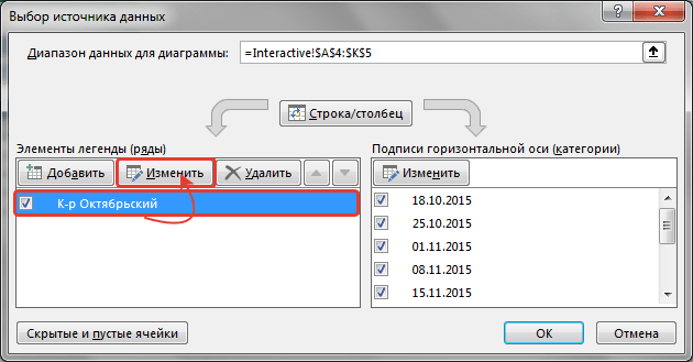

in field Series name enter = Interactive! $ B $ 11

in field Series values enter: = Interactive! _forchart

tip: this field initially contains a direct link: = Interactive! $ B $ 5: $ K $ 5. In order not to miss anything, you just need to replace the cell addresses with the named range that you created earlier - _forchart: = Interactive! $ B $ 5: $ K $ 5 => = Interactive! _forchart
the exclamation mark and possible other marks should be left.

Press OK twice. That's it, our diagram is ready. Now you can select a name from the drop-down list and the chart will change its values ​​to the sales of the selected outlet.
Download example:

(47.5 KiB, 1,017 downloads)

Did the article help? Share the link with your friends! Video lessons

("Bottom bar" :( "textstyle": "static", "textpositionstatic": "bottom", "textautohide": true, "textpositionmarginstatic": 0, "textpositiondynamic": "bottomleft", "textpositionmarginleft": 24, " textpositionmarginright ": 24," textpositionmargintop ": 24," textpositionmarginbottom ": 24," texteffect ":" slide "," texteffecteasing ":" easeOutCubic "," texteffectduration ": 600," texteffectslidedirection ":" left "," texteffectslidedistance " : 30, "texteffectdelay": 500, "texteffectseparate": false, "texteffect1": "slide", "texteffectslidedirection1": "right", "texteffectslidedistance1": 120, "texteffecteasing1": "easeOutCubic", "texteffectduration1": 600 , "texteffectdelay1": 1000, "texteffect2": "slide", "texteffectslidedirection2": "right", "texteffectslidedistance2": 120, "texteffecteasing2": "easeOutCubic", "texteffectduration2": 600, "texteffectdelay2": 1500 textcss ":" display: block; padding: 12px; text-align: left; "," textbgcss ":" display: block; position: absolute; top: 0px; left: 0px; width: 100%; height: 100% ; background-color: # 333333; opacity: 0.6; filter: a lpha (opacity = 60); "," titlecss ":" display: block; position: relative; font: bold 14px \ "Lucida Sans Unicode \", \ "Lucida Grande \", sans-serif, Arial; color: #fff; "," descriptioncss ":" display: block; position: relative; font: 12px \ "Lucida Sans Unicode \", \ "Lucida Grande \", sans-serif, Arial; color: #fff; margin-top: 8px; "," buttoncss ":" display: block; position: relative; margin-top: 8px; "," texteffectresponsive ": true," texteffectresponsivesize ": 640," titlecssresponsive ":" font-size: 12px; "," descriptioncssresponsive ":" display: none! important; "," buttoncssresponsive ": "", "addgooglefonts": false, "googlefonts": "", "textleftrightpercentforstatic": 40))

Information is perceived more easily if it is presented visually. One way to present reports, plans, metrics, and other types of business material is through graphs and charts. In analytics, these are indispensable tools.

There are several ways to build a graph in Excel based on table data. Each of them has its own advantages and disadvantages for a particular situation. Let's consider everything in order.

The simplest schedule of changes

A graph is needed when it is necessary to show changes in data. Let's start with a simple diagram to show events over time.

Let's say we have data on the company's net profit for 5 years:

* Figures are conditional, for educational purposes.

Go to the "Insert" tab. Several types of charts are offered:

We select "Graph". In the pop-up window - its appearance. When you hover the cursor over a particular type of chart, a hint is shown: where is it better to use this chart, for what data.

Chosen - copied the table with data - pasted into the chart area. It turns out this option:

The horizontal straight line (blue) is not needed. Just select it and delete it. Since we have one curve, we also remove the legend (to the right of the graph). To clarify the information, we sign the markers. On the tab "Data Signatures" we determine the location of the numbers. In the example - on the right.

Let's improve the image by labeling the axes. "Layout" - "Name of the axes" - "Name of the main horizontal (vertical) axis":

The title can be removed, moved to the chart area, above it. Change style, fill, etc. All manipulations are on the "Chart Title" tab.

Instead of the serial number of the reporting year, we need exactly the year. Select the values ​​of the horizontal axis. Right-click - "Select data" - "Change labels of the horizontal axis". In the tab that opens, select a range. In the data table, the first column. As shown in the picture below:

We can leave the graph as it is. And we can make a fill, change the font, move the diagram to another sheet ("Constructor" - "Move the diagram").



Graph with two or more curves

Let's say we need to show not only net profit, but also the value of assets. More data:

But the principle of construction remained the same. Only now it makes sense to leave the legend. Since we have 2 curves.

Adding a second axis

How to add a second (additional) axis? When the units are the same, use the instructions above. If you want to show different types of data, you need an auxiliary axis.

First, we build the graph as if we have the same units of measurement.

Select the axis for which we want to add an auxiliary one. Right mouse button - "Data series format" - "Row parameters" - "Along auxiliary axis".

Press "Close" - the second axis appears on the chart, which "adjusted" to the curve data.

This is one way. There is another - changing the type of chart.

Right-click on the line that needs an additional axis. Select "Change chart type for series".

Determine the view for the second data series. In the example, a bar chart.

Just a few clicks - an additional axis for another type of measurement is ready.

Building a graph of functions in Excel

All work consists of two stages:

1. Creation of a table with data.
2. Building a graph.

Example: y = x (√x - 2). Step - 0.3.

We draw up a table. The first column is the X value. We use the formulas. The value of the first cell is 1. The second: = (name of the first cell) + 0.3. Select the lower right corner of the cell with the formula - drag down as much as necessary.

In column Y we write the formula for calculating the function. In our example: = A2 * (ROOT (A2) -2). Press "Enter". Excel calculated the value. "Multiply" the formula across the entire column (by pulling the lower-right corner of the cell). The data table is ready.

Go to a new sheet (you can stay on this - put the cursor in a free cell). "Insert" - "Diagram" - "Scatter". Choose the type you like. We click on the chart area with the right mouse button - "Select data".

Select the X values ​​(first column). And click "Add". The "Edit Series" window opens. We set the name of the row - function. The X-values ​​are the first column of the data table. Y values ​​are second.

Click OK and admire the result.

The Y-axis is okay. There are no values ​​on the x-axis. Only point numbers are provided. This needs to be fixed. It is necessary to sign the axes of the graph in excel. Right mouse button - "Select data" - "Change labels of the horizontal axis". And select the range with the desired values ​​(in the table with data). The schedule becomes what it should be.

Overlay and combine graphs

It is not difficult to create two graphs in Excel. Let's combine two graphs of functions in Excel on one field. Add to the previous one Z = X (√x - 3). Data table:

Select the data and paste it into the chart field. If something is wrong (the names of the rows are wrong, the numbers on the axis are incorrectly reflected), edit it through the "Select data" tab.

And here are our 2 graphs of functions in one field.

Dependency graphs

The data in one column (row) depends on the data in another column (row).

You can build a graph of the dependence of one column on another in Excel as follows:

Conditions: A = f (E); B = f (E); C = f (E); D = f (E).

Choosing a chart type. Point. With smooth curves and markers.

Data selection - "Add". The row name is A. The X values ​​are the A values. The Y values ​​are the E values. Add again. The row name is B. The X values ​​are the data in column B. The Y values ​​are the data in column E. And by this principle, the entire table.

Likewise, you can build donut, bar, bar, bubble, stock, and more. Excel's capabilities are varied. Enough to visualize different types of data.

If your Word document contains a lot of tabular data, then you can visualize it using graphs. The material with graphs will be more visual and it will be more interesting to study it.

It may seem that plotting charts is a difficult task that will take a lot of time, but it is not. The Word text editor has built-in tools that allow you to quickly turn any tabular data into beautiful and understandable graphics.

In this article, we will show you how to make a graph in a text editor Word. In this case, we will consider both modern versions of the editor (Word 2007, 2010, 2013 and 2016) and old ones (Word 2003).

How to make a graph in Word 2007, 2010, 2013 or 2016

In order to make a graph in Word 2007, 2010, 2013 or 2016, place the cursor in the place where the graph should be, go to the "Insert" tab and click on the "" button there.

As a result, a window with a list of all available chart templates will open in front of you. Here you can choose a template to create a bar, pie, line, scatter, stock, and other types of charts. For creating charts, there is a separate group of templates called "Charts" in which several options are available. Select one of them and click on the "OK" button to start setting up the schedule.

After clicking on the "OK" button, a graph will appear in the selected place of the Word document. At the same time, an Excel document will open, in which you need to enter the data for building a graph. The Excel document will have a small table with a blue border. This table is related to the graph that appeared in the document. Therefore, any changes to this table will immediately affect the graph in the Word document.

To customize the schedule, you need to edit the table in Excel. To do this, insert your own column and row names, as well as the data in the cells. In order to increase the number of columns or rows, drag with the mouse the lower right corner of the blue frame that frames the data table.

If you already have a table with data for the graph in your Word document, then you can simply transfer it to Excel. To do this, select the table in Word with the mouse, copy it using Ctrl-C, then select the table in Excel with the mouse, and paste the data using Ctrl-V.

After you have entered the necessary data for the graph, the Excel table window can be simply closed by clicking on the button with the cross. Then you can continue working with the Word document.

If necessary, you can later edit the schedule, for example, change existing values ​​or add new ones. To do this, select the graph with the mouse, go to the "Constructor" tab and click on the "Change data" button.

After that, an Excel window will appear in which you can edit the data and thus change the graph.

How to make a graph in Word 2003

If you are using Word 2003, then in order to create a graph you need to use the "Insert - Chart" menu.

After that, a diagram will appear in the Word 2003 document and a small window for data entry will open.

In order to make a graph, not a diagram, right-click on the diagram and select "Diagram type".

This will open a window with a list of available chart types. Here you need to select "Schedule" and save the settings by clicking on the "OK" button.

After that, you need to enter the data into the table. To do this, double-click the left mouse button on the graph and fill in the table that opens.

After filling out the table, you will receive the schedule you need.